This chapters main concern is the analysis of the effects of the 14 week intervention of 2 x 45 minutes of remedial physical education implemented in the SMaRTER study described in Chapter 2. Improvements of physical fitness and executive function were expected for children who participated in the additional physical fitness compared to a passive control group.
3.2 Statistical analysis
The SMaRTER study implemented a cross-over design with control and intervention groups and pretest and multiple posttest assessments (see Section 2.2). The critical statistic concerns is a Group x Time interaction, with the expectation that children who participate in the additional remedial physical fitness interventions show larger physical fitness and executive function improvements from pre to posttest assessments compared to children of the control group.
The cross-over design was primarily adopted to also enable control children to benefit from possible intervention advantages in a time-delayed manner. The design also allowed for a second test of the primary research hypothesis. If there was an intervention benefit in the first period, it is expected that children in the control group will catch up. Of course, other outcomes are possible depending on whether the group doing the first intervention maintains or increases intervention benefits.
The study also allowed for an evaluation of long-term benefits of the intervention plan. There were additional tests at the beginning of fifth and sixth grade (see Figure 2.1). Due to dropouts, the number of children decreased from the first posttest to the second posttest to long-term follow-up tests (see Figure 2.9). To keep statistical power as large as possible, we tested these hypotheses with three separate linear mixed models (LMMs):
Intervention model 1 (INT M1): first intervention period only
Intervention model 2 (INT M2): pooled intervention periods for both groups1
Intervention model 3 (INT M3): middle and long term intervention-related effects
Specifically, we excluded dropout children for each model (i.e., INT M1 = t0 - t1, INT M2 = t0 - t3, INT M3 = t0 - t8; see Figure 3.1).
Figure 3.1: Dropout with depiction of included children in different intervention models; N = number of assessed participants; INT M1 = Intervention model 1; INT M2 = Intervention model 2; INT M3 = Intervention model 3
For each of the three intervention models, main effects of Group and Time, as well as their interaction were examined with two separate LMMs, one for four tests of physical fitness (i.e., standing long jump, 20 m sprint, 6 min run, and star run) and one for five tests of executive function (i.e., trail making test version A, trail making test version B, digit symbol substitution test, Simon task congruent condition, & Simon task incongruent condition). Components of physical fitness and executive function included in both LMMS were z-transformed (see Appendix Section 8.1.4, and Section 8.1.5) and set as factor levels of Test in each LMM.
Age (centered at 9.3 years), gender, and body mass index (BMI; centered at 17.9 kg/m² for girls and 19.8 kg/m² for boys; see Section 2.7), as well as proximity to Berlin (Kliegl & Teich, 2022) were added as fixed effect control covariates. Significance of covariates was tested using log likelihood ratio tests (LRT) that compared LMMs with and without covariates. All covariates that did not significantly improve LMMs fit were removed from the LMM.
Child was specified as a random factor. Thus, LMMs take into account individual differences between children. Successive difference contrasts were set for the variables Test, Time, Group, Gender, and Berlin Proximity.
3.3 Intervention model 1: First intervention period
Model selection is documented in the Appendix Section 8.3.1.1. For the analysis of intervention effects on physical fitness, Group and Time were included in the fixed factor structure nested within physical fitness Test. In addition, BMI was also included in the nested structure.
m1.6_emo_bmi <-lmer(zScore ~0+ Test/(Group * Time + bmi_c) + (1| Child), data = data_m1_emo, REML =FALSE, control =lmerControl(calc.derivs =FALSE))
3.3.1.2 Results
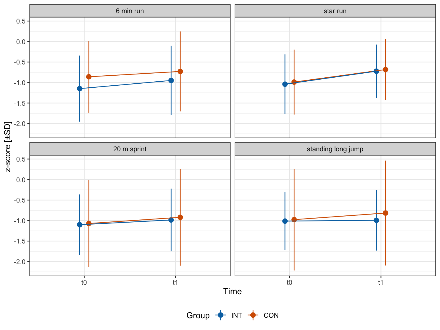
The LMM revealed significant Time-related improvements for star run (β = .31; SE = .1; z = 3.13; p = .002). In addition, effects of BMI were significant for 6 min run (β = -.09; SE = .02; z = -5.27; p < .001), 20 m sprint (β = -.06; SE = .02; z = -3.31; p = .001), and standing long jump (β = -.04; SE = .02; z = -2.09; p = .038), with a lower BMI being associated with better performances. However, there was no evidence for interactions between Time and Group for any of the Tests. Results are presented in Table 3.1 and illustrated in Figure 3.2. Means and standard deviations are reported in the Appendix Section 8.3.1.2.
Code
data_m1_emo |>mutate(Group=ifelse(Group=="CON-INT","CON","INT"),Test=case_when(Test=="Run"~"6 min run", Test=="Star_r"~"star run", Test=="S20_r"~"20 m sprint", Test=="SLJ"~"standing long jump"),Test=factor(Test, levels=c("6 min run", "star run", "20 m sprint", "standing long jump"))) |>group_by(Group, Test, Time) |>summarise(m =mean(zScore),sd=sd(zScore)) |>ggplot(aes(x=Time, y=m, colour= Group, group=Group))+geom_pointrange(aes(ymin=m-sd,ymax=m+sd), position=position_dodge(-0.2)) +geom_line(position=position_dodge(-0.2))+scale_colour_manual(breaks =c("INT", "CON"), values =c(cbPalette)) +facet_wrap(Test~., nrow=2) +ylab("z-score [±SD]") +theme_bw() +theme(legend.position="bottom")
Figure 3.2: Physical fitness plots for the first intervention period CON = control group, INT = intervention group.
Table 3.1: Results of LMM for physical fitness for the first intervention period
Predictors
Est.
SE
z
p
Test [Run]
-0.93
0.09
-10.91
<0.001
Test [Star_r]
-0.86
0.09
-10.05
<0.001
Test [S20_r]
-1.02
0.09
-12.04
<0.001
Test [SLJ]
-0.95
0.09
-11.23
<0.001
Test [Run] : Group2-1
-0.21
0.17
-1.22
0.224
Test [Star_r] : Group2-1
-0.05
0.17
-0.30
0.761
Test [S20_r] : Group2-1
-0.02
0.17
-0.11
0.909
Test [SLJ] : Group2-1
-0.09
0.17
-0.55
0.580
Test [Run] : Time2-1
0.19
0.10
1.92
0.056
Test [Star_r] : Time2-1
0.31
0.10
3.15
0.002
Test [S20_r] : Time2-1
0.15
0.10
1.51
0.131
Test [SLJ] : Time2-1
0.10
0.10
0.99
0.323
Test [Run] : bmi_c
-0.09
0.02
-5.27
<0.001
Test [Star_r] : bmi_c
0.01
0.02
0.42
0.673
Test [S20_r] : bmi_c
-0.06
0.02
-3.31
0.001
Test [SLJ] : bmi_c
-0.04
0.02
-2.09
0.038
Test [Run] : Group2-1 * Time2-1
0.08
0.20
0.41
0.683
Test [Star_r] : Group2-1 * Time2-1
0.01
0.20
0.03
0.977
Test [S20_r] : Group2-1 * Time2-1
-0.03
0.20
-0.15
0.879
Test [SLJ] : Group2-1 * Time2-1
-0.15
0.20
-0.75
0.454
Random Effects
σ2
0.34
τ00Child
0.34
ICC
0.50
N Child
72
Observations
561
Marginal R2 / Conditional R2
0.123 / 0.559
Run = 6 min run, Star_r = star run, S20_r = 20 m sprint, SLJ = standing long jump, bmi_c = gender-specific zero-centered body mass index, Est. = estimate; SE = standar error
3.3.2 Executive function
3.3.2.1 Model fitting
Model selection is documented in the Appendix Section 8.3.2.1. For the analysis of intervention effects on executive function, Group and Time were included in the structure of fixed factors nested in executive function Test. In addition, gender was included in the fixed effects structure.
m1.5_cog_gender <-lmer(zScore ~0+ Test/(Group * Time) + gender + (1| Child), data = data_m1_cog, REML =FALSE, control =lmerControl(calc.derivs =FALSE))
3.3.2.2 Results
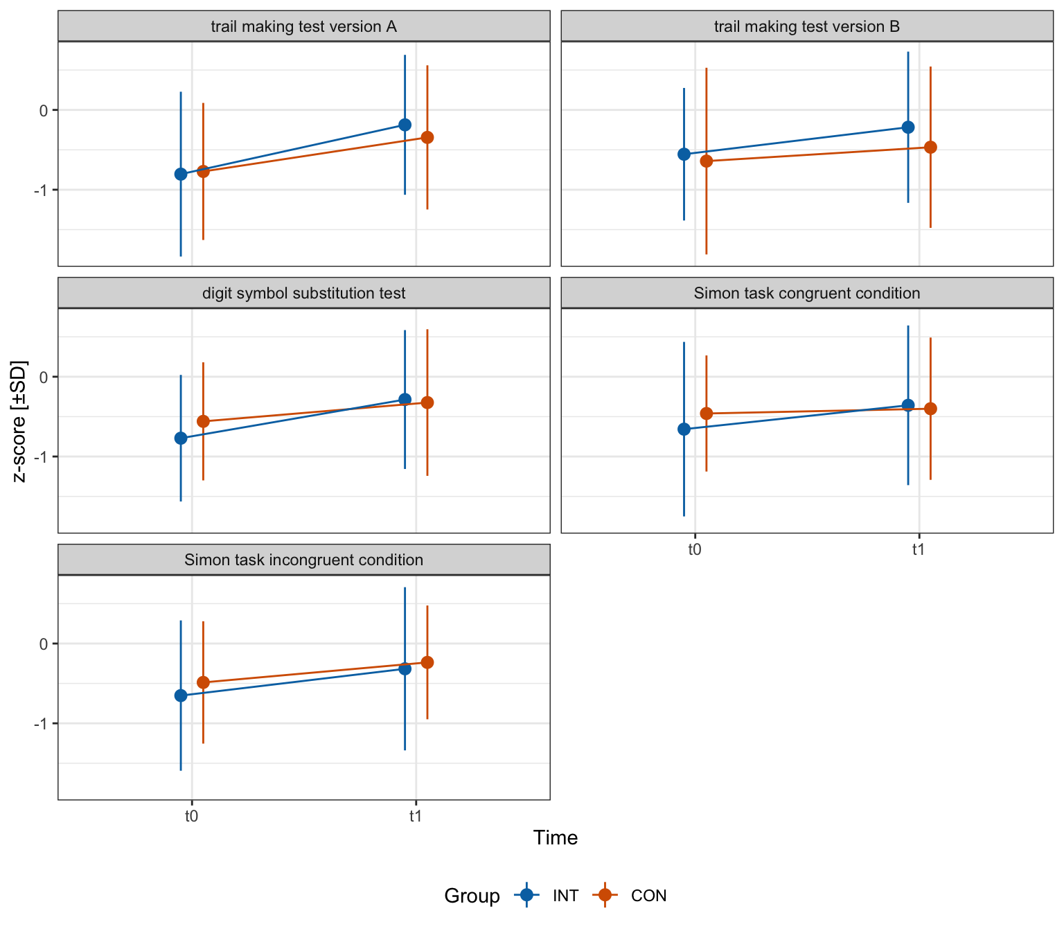
The LMM revealed a significant gender-related effect (β = .33; SE = .13; z = 2.53; p = .012), with better overall executive function performances in boys compared to girls. Overall, Time-related improvements were found for trail making test version A (β = .52; SE = .13; z = 4.05; p < .001), trail making test version B (β = .25; SE = .13; z = 1.97; p = .050), digit symbol substitution test (β = .36; SE = .13; z = 2.78; p = .006), and Simon task incongruent condition (β = .29; SE = .13; z = 2.26; p = .024). However, there was no evidence for interactions between Time and Group for any included executive function Tests. The results are presented in Table 3.2 and mapped in Figure 3.3. Means and standard deviations are reported in the Appendix Section 8.3.2.2.
Code
data_m1_cog |>mutate(Group=ifelse(Group=="CON-INT","CON","INT"),Test=case_when(Test=="TMTa"~"trail making test version A", Test=="TMTb"~"trail making test version B", Test=="DSST"~"digit symbol substitution test", Test=="SC"~"Simon task congruent condition", Test=="SI"~"Simon task incongruent condition"),Test=factor(Test, levels=c("trail making test version A", "trail making test version B", "digit symbol substitution test", "Simon task congruent condition", "Simon task incongruent condition"))) |>group_by(Group, Test, Time) |>summarise(m =mean(zScore),sd=sd(zScore)) |>ggplot(aes(x=Time, y=m, colour=Group, group=Group))+geom_pointrange(aes(ymin=m-sd, ymax=m+sd), position=position_dodge(-0.2)) +geom_line(position=position_dodge(-0.2))+scale_colour_manual(breaks =c("INT", "CON"), values =c(cbPalette)) +facet_wrap(Test~., nrow=3) +ylab("z-score [±SD]") +theme_bw() +theme(legend.position="bottom")
Figure 3.3: Executive function performance plots for the first intervention period, CON = control group, INT = intervention group
Table 3.2: Results of LMM for executive function performances for the first intervention period
Predictors
Est.
SE
z
p
Test [TMTa]
-0.54
0.09
-6.31
<0.001
Test [TMTb]
-0.49
0.09
-5.65
<0.001
Test [DSST]
-0.50
0.09
-5.82
<0.001
Test [SC]
-0.49
0.09
-5.64
<0.001
Test [SI]
-0.44
0.09
-5.11
<0.001
gender2-1
0.33
0.13
2.53
0.012
Test [TMTa] : Group2-1
-0.01
0.17
-0.05
0.962
Test [TMTb] : Group2-1
0.10
0.17
0.57
0.571
Test [DSST] : Group2-1
-0.16
0.17
-0.91
0.365
Test [SC] : Group2-1
-0.15
0.17
-0.85
0.396
Test [SI] : Group2-1
-0.19
0.17
-1.11
0.266
Test [TMTa] : Time2-1
0.52
0.13
4.05
<0.001
Test [TMTb] : Time2-1
0.25
0.13
1.97
0.050
Test [DSST] : Time2-1
0.36
0.13
2.78
0.006
Test [SC] : Time2-1
0.18
0.13
1.37
0.172
Test [SI] : Time2-1
0.29
0.13
2.26
0.024
Test [TMTa] : Group2-1 * Time2-1
0.13
0.26
0.52
0.602
Test [TMTb] : Group2-1 * Time2-1
0.11
0.26
0.42
0.678
Test [DSST] : Group2-1 * Time2-1
0.19
0.26
0.75
0.456
Test [SC] : Group2-1 * Time2-1
0.18
0.26
0.71
0.479
Test [SI] : Group2-1 * Time2-1
0.03
0.26
0.11
0.916
Random Effects
σ2
0.57
τ00Child
0.23
ICC
0.29
N Child
72
Observations
705
Marginal R2 / Conditional R2
0.072 / 0.344
TMTa = trail making test version A, TMTb = trail making test version B, DSST = digit symbol substitution test, SC = Simon task congruent condition, SI = Simon task incongruent condition, Est. = estimate; SE = standar error
3.4 Intervention model 2: Pooled intervention period
Model selection is documented in the Appendix Section 8.3.3.1. For the analysis of intervention effects of physical fitness, Group (pooled) and Time (pooled) nested under the factor levels of Test. In addition, BMI was included in the nested structure of Test.
m2.6_emo_bmi <-lmer(zScore ~0+ Test/(Group_pooled * Time_pooled + bmi_c) + (1| Child), data = data_m2_emo, REML =FALSE, control =lmerControl(calc.derivs =FALSE))
3.4.1.2 Results
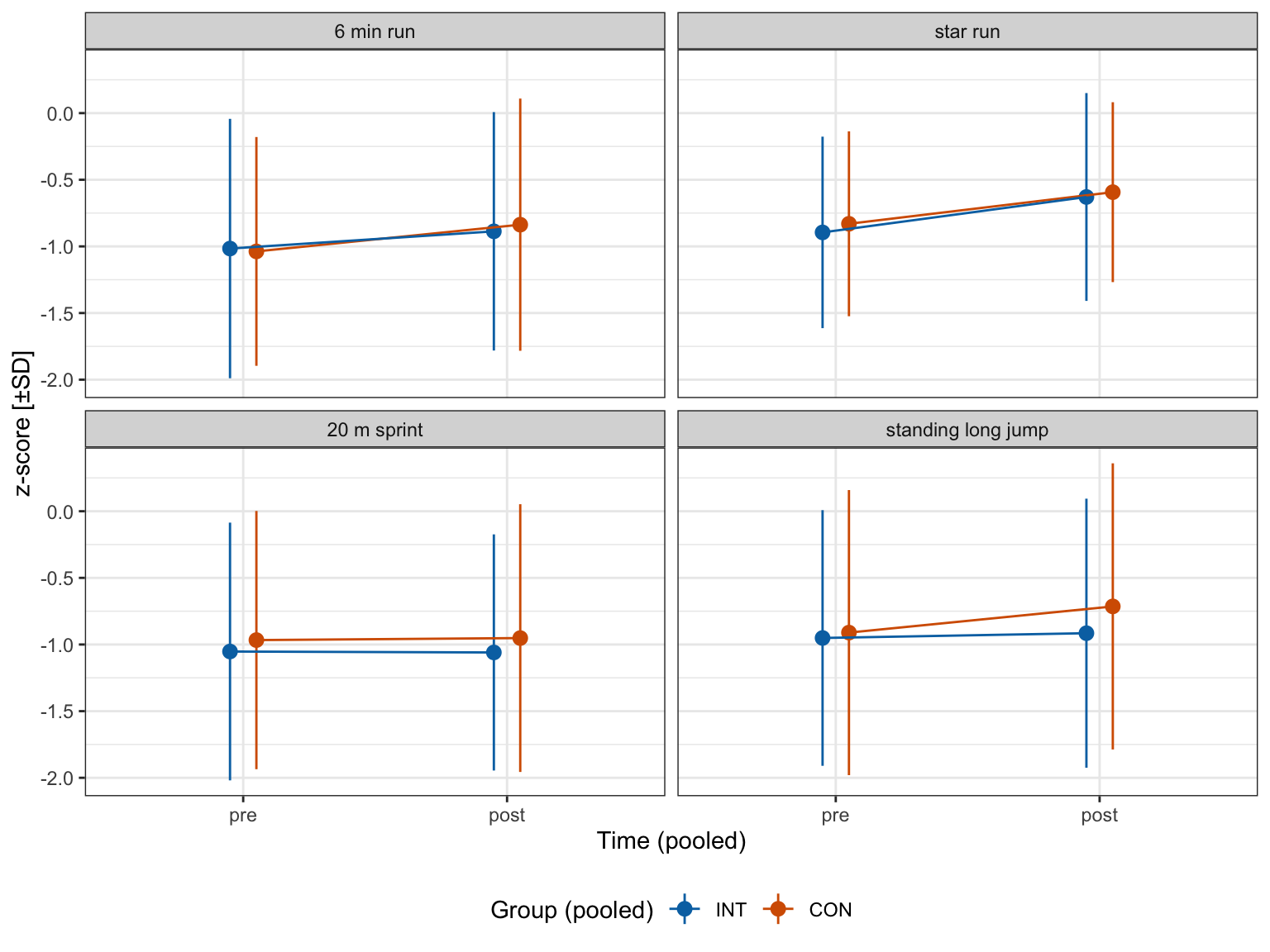
LMM revealed significant overall Time-related (pooled) improvements for 6 min run (β = .2; SE = .08; z = 2.54; p = .011) and star run (β = .27; SE = .08; z = 3.45; p = .001). For 6 min run (β = -.09; SE = .02; z = -5.59; p < .001), star run (β = -.05; SE = .02; z = -3.18; p = .002), and standing long jump (β = -.04; SE = .02; z = -2.5; p = .013), the LMM revealed lower BMI to be associated with better performances. However, significant interactions of Time (pooled) and Group (pooled) were not found for any of the implemented Tests. Results are presented in Table 3.3 and depicted in Figure 3.4. Means and standard deviations are reported in the Appendix Section 8.3.3.2.
Code
data_m2_emo |>mutate(Test=case_when(Test=="Run"~"6 min run", Test=="Star_r"~"star run", Test=="S20_r"~"20 m sprint", Test=="SLJ"~"standing long jump"),Test=factor(Test, levels=c("6 min run", "star run", "20 m sprint", "standing long jump"))) |>group_by(Group_pooled, Test, Time_pooled) |>summarise(m =mean(zScore),sd=sd(zScore)) |>ggplot(aes(x=Time_pooled, y=m, colour= Group_pooled, group=Group_pooled))+geom_pointrange(aes(ymin=m-sd,ymax=m+sd), position=position_dodge(-0.2)) +geom_line(position=position_dodge(-0.2))+scale_colour_manual(breaks =c("INT", "CON"), values =c(cbPalette)) +facet_wrap(Test~., nrow=2) +labs(x="Time (pooled)",y="z-score [±SD]",colour="Group (pooled)") +theme_bw() +theme(legend.position="bottom")
Figure 3.4: Physical fitness plots for the pooled intervention period, CON = control group, INT = intervention group
Table 3.3: Results of LMM for physical fitness for the pooled intervention period
Predictors
Est.
SE
z
p
Test [Run]
-0.94
0.08
-11.35
<0.001
Test [Star_r]
-0.73
0.08
-8.85
<0.001
Test [S20_r]
-1.00
0.08
-12.13
<0.001
Test [SLJ]
-0.87
0.08
-10.51
<0.001
Test [Run] : Group_pooled2-1
0.02
0.08
0.26
0.793
Test [Star_r] : Group_pooled2-1
-0.04
0.08
-0.46
0.645
Test [S20_r] : Group_pooled2-1
-0.07
0.08
-0.97
0.333
Test [SLJ] : Group_pooled2-1
-0.10
0.08
-1.33
0.184
Test [Run] : Time_pooled2-1
0.20
0.08
2.54
0.011
Test [Star_r] : Time_pooled2-1
0.27
0.08
3.45
0.001
Test [S20_r] : Time_pooled2-1
0.04
0.08
0.53
0.597
Test [SLJ] : Time_pooled2-1
0.15
0.08
1.92
0.055
Test [Run] : bmi_c
-0.09
0.02
-5.59
<0.001
Test [Star_r] : bmi_c
0.00
0.02
0.15
0.884
Test [S20_r] : bmi_c
-0.05
0.02
-3.18
0.002
Test [SLJ] : bmi_c
-0.04
0.02
-2.50
0.013
Test [Run] : Group_pooled2-1 * Time_pooled2-1
0.03
0.15
0.16
0.871
Test [Star_r] : Group_pooled2-1 * Time_pooled2-1
0.06
0.15
0.39
0.695
Test [S20_r] : Group_pooled2-1 * Time_pooled2-1
0.02
0.15
0.11
0.910
Test [SLJ] : Group_pooled2-1 * Time_pooled2-1
-0.13
0.15
-0.83
0.407
Random Effects
σ2
0.37
τ00Child
0.35
ICC
0.49
N Child
66
Observations
1019
Marginal R2 / Conditional R2
0.106 / 0.540
Run = 6 min run, Star_r = star run, S20_r = 20 m sprint, SLJ = standing long jump, bmi_c = gender-specific zero-centered body mass index, Est. = estimate; SE = standar error
3.4.2 Executive function
3.4.2.1 Model fitting
Model selection is documented in the Appendix Section 8.3.4.1. For the analysis of intervention effects on executive function, Group (pooled) and Time (pooled) were nested within the factor levels of Test. In addition, age was also included in the fixed effects structure.
m2.5_cog_gender <-lmer(zScore ~0+ Test/(Group_pooled * Time_pooled) + a1 + (1| Child), data = data_m2_cog, REML =FALSE, control =lmerControl(calc.derivs =FALSE))
3.4.2.2 Results
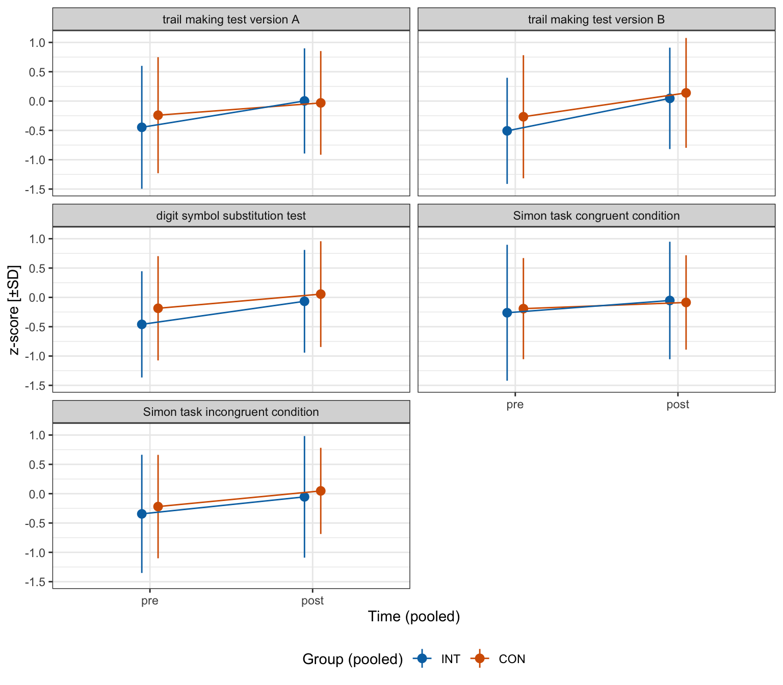
LMM revealed overall age-related improvements in executive function (β = .89; SE = .07; z = 13.08; p < .001). However, no evidence for significant effects of Time (pooled), Group (pooled), or interactions of Time (pooled) and Group (pooled) were found for any of the implemented Tests. Results are presented in Table 3.4 and depicted in Figure 3.5. Means and standard deviations are reported in the Appendix Section 8.3.4.2.
Code
data_m2_cog |>mutate(Test=case_when(Test=="TMTa"~"trail making test version A", Test=="TMTb"~"trail making test version B", Test=="DSST"~"digit symbol substitution test", Test=="SC"~"Simon task congruent condition", Test=="SI"~"Simon task incongruent condition"),Test=factor(Test, levels=c("trail making test version A", "trail making test version B", "digit symbol substitution test", "Simon task congruent condition", "Simon task incongruent condition"))) |>group_by(Group_pooled, Test, Time_pooled) |>summarise(m =mean(zScore),sd=sd(zScore)) |>ggplot(aes(x=Time_pooled, y=m, colour=Group_pooled, group=Group_pooled))+geom_pointrange(aes(ymin=m-sd, ymax=m+sd), position=position_dodge(-0.2)) +geom_line(position=position_dodge(-0.2))+scale_colour_manual(breaks =c("INT", "CON"), values =c(cbPalette)) +facet_wrap(Test~., nrow=3) +labs(x="Time (pooled)",y="z-score [±SD]",colour="Group (pooled)") +theme_bw() +theme(legend.position="bottom")
Figure 3.5: Executive function plots for the pooled intervention period, CON = control group, INT = intervention group
Table 3.4: Results of the LMM for executive function performance for the pooled intervention period
Predictors
Est.
SE
z
p
Test [TMTa]
-0.16
0.10
-1.68
0.093
Test [TMTb]
-0.13
0.10
-1.35
0.177
Test [DSST]
-0.15
0.10
-1.53
0.127
Test [SC]
-0.13
0.10
-1.35
0.178
Test [SI]
-0.12
0.10
-1.29
0.198
a1
0.89
0.07
13.08
<0.001
Test [TMTa] : Group_pooled2-1
-0.04
0.09
-0.45
0.649
Test [TMTb] : Group_pooled2-1
-0.12
0.09
-1.33
0.185
Test [DSST] : Group_pooled2-1
-0.15
0.09
-1.67
0.095
Test [SC] : Group_pooled2-1
0.02
0.09
0.25
0.804
Test [SI] : Group_pooled2-1
-0.07
0.09
-0.78
0.433
Test [TMTa] : Time_pooled2-1
0.00
0.09
0.00
0.996
Test [TMTb] : Time_pooled2-1
0.15
0.09
1.59
0.112
Test [DSST] : Time_pooled2-1
-0.01
0.09
-0.12
0.902
Test [SC] : Time_pooled2-1
-0.17
0.09
-1.79
0.074
Test [SI] : Time_pooled2-1
-0.05
0.09
-0.50
0.614
Test [TMTa] : Group_pooled2-1 * Time_pooled2-1
0.22
0.18
1.21
0.228
Test [TMTb] : Group_pooled2-1 * Time_pooled2-1
0.13
0.18
0.70
0.483
Test [DSST] : Group_pooled2-1 * Time_pooled2-1
0.13
0.18
0.73
0.468
Test [SC] : Group_pooled2-1 * Time_pooled2-1
0.08
0.18
0.42
0.671
Test [SI] : Group_pooled2-1 * Time_pooled2-1
-0.00
0.18
-0.02
0.988
Random Effects
σ2
0.54
τ00Child
0.48
ICC
0.47
N Child
66
Observations
1289
Marginal R2 / Conditional R2
0.238 / 0.594
TMTa = trail making test version A, TMTb = trail making test version B, DSST = digit symbol substitution test, SC = Simon task congruent condition, SI = Simon task incongruent condition, a1 = zero-centered age, Est. = estimate; SE = standar error
Model selection is documented in the Appendix Section 8.3.5.1. For the analysis of long-term intervention effects on physical fitness, Group and Time were included in the fixed factor structure, which was nested within Test. In addition, BMI and Berlin proximity were included in the nested structure of Test.
m3.6_emo_bmibp <-lmer(zScore ~0+ Test/(Group * Time + bmi_c + bp) + (1| Child), data = data_m3_emo, REML =FALSE, control =lmerControl(calc.derivs =FALSE))
3.5.1.2 Results
The LMM revealed a significant overall Time-related improvement for star run between t0 and t1 (β = .3; SE = .15; z = 2.07; p = .039) and t2 and t3 (β = .32; SE = .15; z = 2.17; p = .030), for 20 m sprint between t6 and t8 (β = .4; SE = .15; z = 2.58; p = .010), and for standing long jump between t6 and t8 (β = .5; SE = .15; z = 3.26; p = .001). Further, analysis revealed significant effects of BMI for 6 min run (β = -.09; SE = .02; z = -5.62; p < .001), and 20 m sprint (β = -.04; SE = .02; z = -2.78; p = .006) with better performances being associated with a lower BMI. Effects of Berlin proximity were found for 6 min run (β = .-81; SE = .3; z = -2.73; p = .006), and standing long jump (β = .-76; SE = .3; z = -2.56; p = .011) with better performances being associated with children living close to Berlin. However, no evidence for interactions of Time and Group were found for any of the implemented Tests. Results are presented in Table 3.5 and depicted in Figure 3.6. Means and standard deviations are reported in the Appendix Section 8.3.5.2.
Code
data_m3_emo |>mutate(Test=case_when(Test=="Run"~"6 min run", Test=="Star_r"~"star run", Test=="S20_r"~"20 m sprint", Test=="SLJ"~"standing long jump"),Test=factor(Test, levels=c("6 min run", "star run", "20 m sprint", "standing long jump"))) |>group_by(Group, Test, Time) |>summarise(m =mean(zScore),sd=sd(zScore)) |>ggplot(aes(x=Time, y=m, colour= Group, group=Group))+geom_pointrange(aes(ymin=m-sd,ymax=m+sd), position=position_dodge(-0.2)) +geom_line(position=position_dodge(-0.2))+scale_colour_manual(breaks =c("INT-CON", "CON-INT"), values =c(cbPalette)) +facet_wrap(Test~., nrow=2) +ylab("z-score [±SD]") +theme_bw() +theme(legend.position="bottom")
Figure 3.6: Physical fitness plots of long-term intervention effects, CON-INT = control condition between t0 and t1 and intervention condition between t2 and t3, INT-CON = intervention condition between t0 and t1 and control condition between t2 and t3
Table 3.5: Results of LMM for physical fitness for the long-term intervention effects
Predictors
Est.
SE
z
p
Test [Run]
-0.88
0.13
-6.87
<0.001
Test [Star_r]
-0.45
0.13
-3.50
<0.001
Test [S20_r]
-0.74
0.13
-5.79
<0.001
Test [SLJ]
-0.46
0.13
-3.58
<0.001
Test [Run] : Group2-1
0.20
0.23
0.87
0.387
Test [Star_r] : Group2-1
0.01
0.23
0.03
0.974
Test [S20_r] : Group2-1
0.39
0.23
1.66
0.097
Test [SLJ] : Group2-1
0.37
0.23
1.61
0.108
Test [Run] : Time2-1
0.14
0.15
0.97
0.332
Test [Star_r] : Time2-1
0.30
0.15
2.07
0.039
Test [S20_r] : Time2-1
0.13
0.15
0.89
0.376
Test [SLJ] : Time2-1
0.03
0.15
0.17
0.862
Test [Run] : Time3-2
-0.16
0.15
-1.08
0.281
Test [Star_r] : Time3-2
-0.11
0.15
-0.75
0.452
Test [S20_r] : Time3-2
0.13
0.15
0.89
0.372
Test [SLJ] : Time3-2
-0.07
0.15
-0.45
0.652
Test [Run] : Time4-3
0.16
0.15
1.06
0.290
Test [Star_r] : Time4-3
0.32
0.15
2.17
0.030
Test [S20_r] : Time4-3
-0.11
0.15
-0.76
0.447
Test [SLJ] : Time4-3
0.26
0.15
1.79
0.074
Test [Run] : Time5-4
-0.02
0.15
-0.16
0.876
Test [Star_r] : Time5-4
0.26
0.15
1.72
0.087
Test [S20_r] : Time5-4
0.29
0.15
1.86
0.063
Test [SLJ] : Time5-4
0.14
0.15
0.89
0.374
Test [Run] : Time6-5
0.15
0.16
0.94
0.346
Test [Star_r] : Time6-5
0.07
0.15
0.45
0.651
Test [S20_r] : Time6-5
0.40
0.15
2.58
0.010
Test [SLJ] : Time6-5
0.50
0.15
3.26
0.001
Test [Run] : bmi_c
-0.09
0.02
-5.62
<0.001
Test [Star_r] : bmi_c
-0.01
0.02
-0.59
0.558
Test [S20_r] : bmi_c
-0.04
0.02
-2.78
0.006
Test [SLJ] : bmi_c
-0.03
0.02
-1.73
0.084
Test [Run] : bp2-1
-0.81
0.30
-2.73
0.007
Test [Star_r] : bp2-1
-0.25
0.30
-0.85
0.393
Test [S20_r] : bp2-1
-0.58
0.30
-1.95
0.052
Test [SLJ] : bp2-1
-0.76
0.30
-2.56
0.011
Test [Run] : Group2-1 * Time2-1
0.49
0.29
1.68
0.094
Test [Star_r] : Group2-1 * Time2-1
0.14
0.29
0.49
0.624
Test [S20_r] : Group2-1 * Time2-1
-0.13
0.29
-0.46
0.646
Test [SLJ] : Group2-1 * Time2-1
-0.02
0.29
-0.08
0.940
Test [Run] : Group2-1 * Time3-2
-0.31
0.30
-1.05
0.293
Test [Star_r] : Group2-1 * Time3-2
0.05
0.29
0.16
0.870
Test [S20_r] : Group2-1 * Time3-2
0.42
0.29
1.44
0.149
Test [SLJ] : Group2-1 * Time3-2
0.12
0.29
0.42
0.674
Test [Run] : Group2-1 * Time4-3
0.04
0.30
0.15
0.881
Test [Star_r] : Group2-1 * Time4-3
0.05
0.29
0.19
0.853
Test [S20_r] : Group2-1 * Time4-3
-0.10
0.29
-0.34
0.735
Test [SLJ] : Group2-1 * Time4-3
0.41
0.29
1.40
0.163
Test [Run] : Group2-1 * Time5-4
0.01
0.31
0.04
0.964
Test [Star_r] : Group2-1 * Time5-4
-0.07
0.31
-0.23
0.816
Test [S20_r] : Group2-1 * Time5-4
0.18
0.31
0.60
0.551
Test [SLJ] : Group2-1 * Time5-4
0.01
0.31
0.02
0.986
Test [Run] : Group2-1 * Time6-5
0.47
0.31
1.53
0.128
Test [Star_r] : Group2-1 * Time6-5
0.13
0.31
0.41
0.679
Test [S20_r] : Group2-1 * Time6-5
-0.00
0.30
-0.01
0.989
Test [SLJ] : Group2-1 * Time6-5
-0.15
0.30
-0.48
0.635
Random Effects
σ2
0.38
τ00Child
0.28
ICC
0.43
N Child
37
Observations
836
Marginal R2 / Conditional R2
0.313 / 0.605
Run = 6 min run, Star_r = star run, S20_r = 20 m sprint, SLJ = standing long jump, bmi_c = gender-specific zero-centered body mass index, Est. = estimate; SE = standar error
3.5.2 Executive function
3.5.2.1 Model fitting
Model selection is documented in the Appendix Section 8.3.6.1. For the analysis of intervention on executive function, Group and Time were included in the fixed factor structure within Test. No other covariates were included in the LMM.
m3.2_cog <-lmer(zScore ~0+ Test/(Group * Time) + (1| Child), data = data_m3_cog, REML =FALSE, control =lmerControl(calc.derivs =FALSE))
3.5.2.2 Results
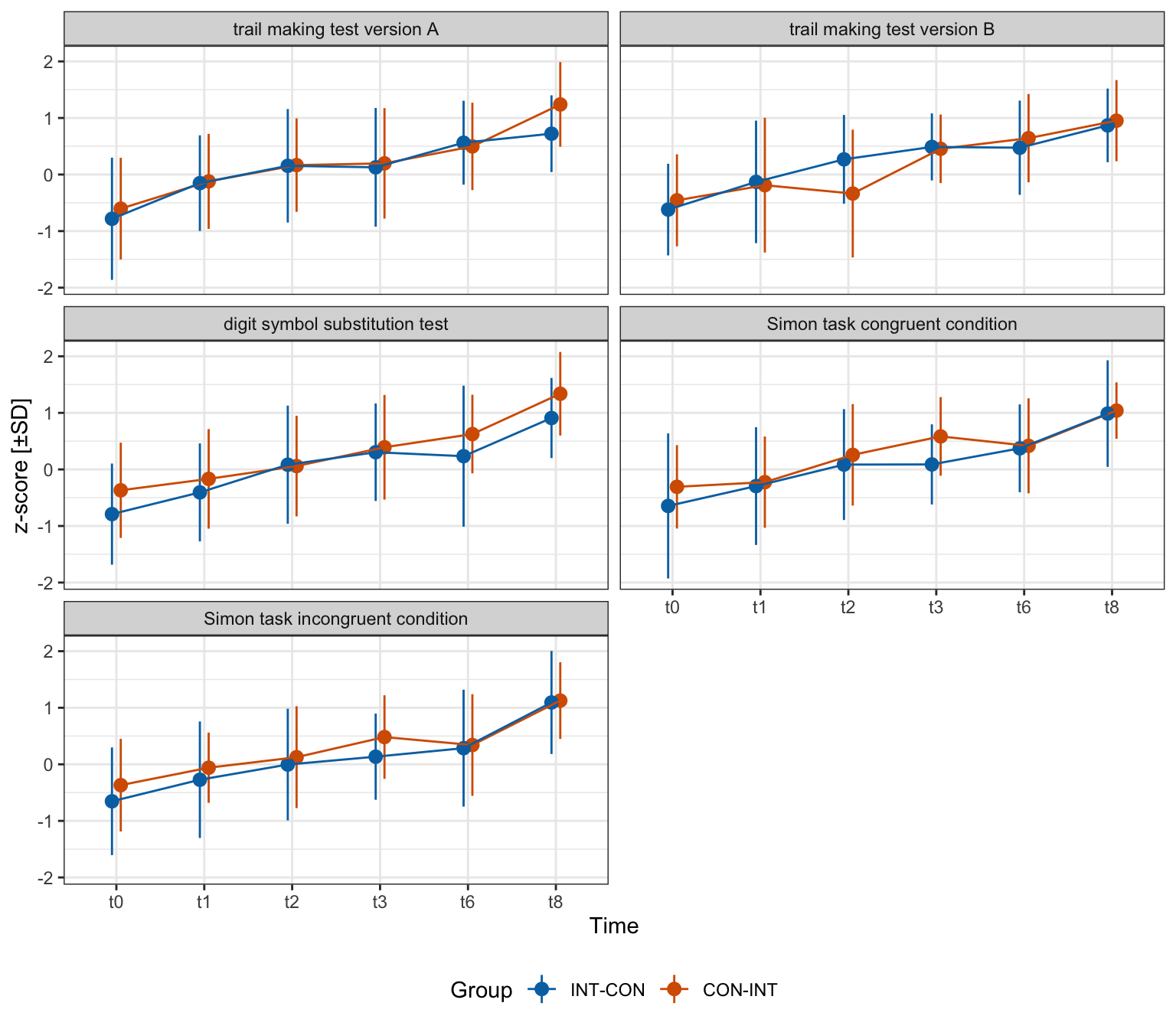
The LMM revealed a significant overall Time-related improvement for trail making test version A between t0 and t1 (β = .55; SE = .16; z = 3.36; p = .001), t3 and t6 (β = .43; SE = .17; z = 2.53; p = .012), and t6 and t8 (β = .40; SE = .17; z = 2.37; p = .018). For trail making test version B, performance improved between t0 and t1 (β = .37; SE = .16; z = 2.27; p = .023), and t2 and t3 (β = .49; SE = .16; z = 3.01; p = .003). For digit symbol substitution test, performance improved between t1 and t2 (β = .37; SE = .16; z = 2.25; p = .025), and t6 and t8 (β = .64; SE = .17; z = 3.81; p < .001). Similarly, for Simon task congruent condition, performance improved between t1 and t2 (β = .44; SE = .16; z = 2.70; p = .007), and t6 and t8 (β = .57; SE = .17; z = 3.37; p = .001); and for Simon task incongruent condition, performance improved between t0 and t1 (β = .34; SE = .16; z = 2.06; p = .039), and t6 and t8 (β = .75; SE = .17; z = 4.42; p < .001). However, there was no evidence for interactions of Time and Group for any of the implemented executive function Tests. Results are presented in Table 3.6 and depicted in Figure 3.7. Means and standard deviations are reported in the Appendix Section 8.3.6.2.
Code
data_m3_cog |>mutate(Test=case_when(Test=="TMTa"~"trail making test version A", Test=="TMTb"~"trail making test version B", Test=="DSST"~"digit symbol substitution test", Test=="SC"~"Simon task congruent condition", Test=="SI"~"Simon task incongruent condition"),Test=factor(Test, levels=c("trail making test version A", "trail making test version B", "digit symbol substitution test", "Simon task congruent condition", "Simon task incongruent condition"))) |>group_by(Group, Test, Time) |>summarise(m =mean(zScore),sd=sd(zScore)) |>ggplot(aes(x=Time, y=m, colour=Group, group=Group))+geom_pointrange(aes(ymin=m-sd, ymax=m+sd), position=position_dodge(-0.2)) +geom_line(position=position_dodge(-0.2))+scale_colour_manual(breaks =c("INT-CON", "CON-INT"), values =c(cbPalette)) +facet_wrap(Test~., nrow=3) +ylab("z-score [±SD]") +theme_bw() +theme(legend.position="bottom")
Figure 3.7: Executive function performance plots of long-term intervention effects, CON-INT = control condition between t0 and t1 and intervention condition between t2 and t3, INT-CON = intervention condition between t0 and t1 and control condition between t2 and t3
Table 3.6: Results of LMM for executive function performance for the long-term intervention effects
Predictors
Est.
SE
z
p
Test [TMTa]
0.17
0.09
1.82
0.069
Test [TMTb]
0.21
0.09
2.18
0.030
Test [DSST]
0.19
0.09
2.00
0.046
Test [SC]
0.20
0.09
2.15
0.032
Test [SI]
0.19
0.09
2.03
0.042
Test [TMTa] : Group2-1
-0.14
0.19
-0.73
0.468
Test [TMTb] : Group2-1
0.03
0.19
0.18
0.860
Test [DSST] : Group2-1
-0.27
0.19
-1.43
0.153
Test [SC] : Group2-1
-0.21
0.19
-1.12
0.263
Test [SI] : Group2-1
-0.19
0.19
-1.03
0.305
Test [TMTa] : Time2-1
0.55
0.16
3.36
0.001
Test [TMTb] : Time2-1
0.37
0.16
2.27
0.023
Test [DSST] : Time2-1
0.28
0.16
1.74
0.081
Test [SC] : Time2-1
0.21
0.16
1.28
0.202
Test [SI] : Time2-1
0.34
0.16
2.06
0.039
Test [TMTa] : Time3-2
0.31
0.16
1.88
0.061
Test [TMTb] : Time3-2
0.13
0.16
0.82
0.411
Test [DSST] : Time3-2
0.37
0.16
2.25
0.025
Test [SC] : Time3-2
0.44
0.16
2.70
0.007
Test [SI] : Time3-2
0.24
0.16
1.45
0.148
Test [TMTa] : Time4-3
-0.01
0.16
-0.08
0.938
Test [TMTb] : Time4-3
0.49
0.16
3.01
0.003
Test [DSST] : Time4-3
0.26
0.16
1.60
0.109
Test [SC] : Time4-3
0.16
0.16
0.98
0.325
Test [SI] : Time4-3
0.24
0.16
1.50
0.135
Test [TMTa] : Time5-4
0.43
0.17
2.53
0.012
Test [TMTb] : Time5-4
0.15
0.17
0.89
0.373
Test [DSST] : Time5-4
0.15
0.17
0.86
0.389
Test [SC] : Time5-4
0.11
0.17
0.68
0.499
Test [SI] : Time5-4
0.06
0.17
0.36
0.719
Test [TMTa] : Time6-5
0.40
0.17
2.37
0.018
Test [TMTb] : Time6-5
0.30
0.17
1.79
0.075
Test [DSST] : Time6-5
0.64
0.17
3.81
<0.001
Test [SC] : Time6-5
0.57
0.17
3.37
0.001
Test [SI] : Time6-5
0.75
0.17
4.42
<0.001
Test [TMTa] : Group2-1 * Time2-1
0.08
0.33
0.25
0.806
Test [TMTb] : Group2-1 * Time2-1
0.15
0.33
0.47
0.637
Test [DSST] : Group2-1 * Time2-1
0.11
0.33
0.35
0.727
Test [SC] : Group2-1 * Time2-1
0.20
0.33
0.61
0.539
Test [SI] : Group2-1 * Time2-1
0.01
0.33
0.02
0.987
Test [TMTa] : Group2-1 * Time3-2
0.09
0.33
0.27
0.789
Test [TMTb] : Group2-1 * Time3-2
0.61
0.33
1.89
0.060
Test [DSST] : Group2-1 * Time3-2
0.33
0.33
1.02
0.309
Test [SC] : Group2-1 * Time3-2
-0.03
0.33
-0.11
0.915
Test [SI] : Group2-1 * Time3-2
0.15
0.33
0.46
0.644
Test [TMTa] : Group2-1 * Time4-3
-0.03
0.33
-0.09
0.931
Test [TMTb] : Group2-1 * Time4-3
-0.54
0.33
-1.66
0.097
Test [DSST] : Group2-1 * Time4-3
-0.08
0.33
-0.25
0.802
Test [SC] : Group2-1 * Time4-3
-0.31
0.32
-0.96
0.335
Test [SI] : Group2-1 * Time4-3
-0.21
0.32
-0.64
0.524
Test [TMTa] : Group2-1 * Time5-4
0.06
0.34
0.19
0.852
Test [TMTb] : Group2-1 * Time5-4
-0.27
0.34
-0.80
0.423
Test [DSST] : Group2-1 * Time5-4
-0.38
0.34
-1.10
0.273
Test [SC] : Group2-1 * Time5-4
0.40
0.34
1.17
0.241
Test [SI] : Group2-1 * Time5-4
0.24
0.34
0.70
0.483
Test [TMTa] : Group2-1 * Time6-5
-0.54
0.34
-1.60
0.110
Test [TMTb] : Group2-1 * Time6-5
0.13
0.34
0.38
0.706
Test [DSST] : Group2-1 * Time6-5
0.00
0.34
0.01
0.991
Test [SC] : Group2-1 * Time6-5
0.03
0.34
0.10
0.921
Test [SI] : Group2-1 * Time6-5
0.06
0.34
0.19
0.849
Random Effects
σ2
0.48
τ00Child
0.25
ICC
0.34
N Child
37
Observations
1062
Marginal R2 / Conditional R2
0.285 / 0.529
TMTa = trail making test version a, TMTb = trail making test version b, DSST = digit symbol substitution test, SC = Simon task congruent condition, SI = Simon task incongruent condition, Est. = estimate; SE = standar error
3.6 Summary of results
The most striking outcome of assessing the effects of the implemented 14-week quantitative remedial physical education intervention on physical fitness and executive function of children with deficits in their physical fitness, was (1) the absence of detectable intervention-related improvements of physical fitness or executive functions in any of the approaches used.
Other results revealed by the LMMs were (2) several improvements over time in all tests of physical fitness and executive functions, (3) interactions between BMI and 6 min run, star run, and standing long jump performances, with better performances in children with a lower BMI, (4) an effect of proximity to Berlin on performance in 6 min run and standing long jump, with children living closer to Berlin performing better, (5) improvements in executive function test performance with age, and (6) gendered differences in executive function test performances, with boys performing better compared to girls.
3.7 Discussion
Regarding the absence of detectable intervention effects, two potential factors hold plausible explanations in relation to the remedial physical education intervention: (1) duration of the intervention period and (2) exercise specificity. A meta-analysis summarising effects of additional physical education found positive effects in cardiorespiratory and muscular fitness, however the study included predominantly studies with intervention periods lasting one year or longer (i.e., 17 out of 20 studies) (García-Hermoso et al., 2020). One of the included studies examined effects of two additional physical education lessons over a 16-week period in adolescents aged 12 to 14 years and found intervention-related effects for shuttle run but not standing long jump and 4 x 10 m shuttle run performances (Ardoy et al., 2011). In another study, additional physical education lessons were implemented for 8 weeks, however, the publication was only available in Spanish and therefore could not be further discussed in this thesis (Lechuga et al., 2012). This could indicate that intervention periods of 14 weeks, as used in the SMaRTER study, might be insufficient to achieve detectable intervention effects.
Studies examining effects of more specific exercises (i.e., exercises that focus on improving specific subcomponents of physical fitness) integrated into existing physical education classes have shown to induce intervention-related benefits compared to regular physical education lessons. For example, studies in which 9- to 10-week plyometric programs were integrated into the physical education curriculum with children aged 8 to 12 years found greater improvements in sprint speed, vertical jump height, standing long jump distance, number of push-ups, and half-mile run performance compared to regular physical education controls2(Faigenbaum & Farrell, 2009; Kotzamanidis, 2006). Similarly, in a study examining effects of an 8-week resistance training program incorporated into physical education in children aged 10 to 12 years, greater intervention-related improvements were found in sit-up and arm bend performances, but not in standing long jump distance, compared to regular physical education3(Viciana et al., 2013). As the SMaRTER study included a comprehensive intervention program aimed at improving several components of physical fitness in children, the respective exercises might have been insufficient to induce intervention-related improvements in physical fitness components. While a 14-week intervention curriculum aimed at improving a specific component of physical fitness could have achieved significant intervention effects, the SMaRTER study was oriented towards bringing general physical fitness of participating children to a level comparable to that of their peers, while offering exercises in a curriculum that was fun and provided a safe community learning experience for participating children (KMK, 1999). Accordingly, implementing the SMaRTER physical education curriculum over a longer period of time (i.e., ≥ one school year) may have resulted in measurable intervention-related improvements in physical fitness and executive function.
A similar dynamic can be observed in studies examining effects of physical education-based interventions on executive function. For example, a review article examining effects of additional physical education on executive function and academic performance predominantly included studies with intervention durations longer than one year (i.e., 3 out of 4 studies) (Garciá-Hermoso et al., 2021). Shorter interventions based on physical education tend to implement training protocols involving some form of high-intensity exercise such as high-intensity interval training (Costigan et al., 2016; Garciá-Hermoso et al., 2021; Martínez-Lopez et al., 2018; Xue et al., 2019). Thus similarly to the lack of detectable intervention-related improvements on physical fitness, the lack of intervention-related effects on executive function in the SMaRTER study may also have attributed to an insufficient intervention period duration or an insufficient training intensity.
Another factor to consider in this discussion would be the inclusion of children with deficits in their physical fitness. In the SMaRTER study, it was hypothesised that children with deficits in their physical fitness would make greater improvements when exposed to additional exercise due to their larger potentials. However, this view is biased by the assumption that deficits in physical fitness are caused by a mere lack of exercise or can at least be properly addressed by additional exercising, thereby neglecting, for example, sociocultural conditions related to children’s physical fitness levels. This will be discussed further in Section 7.3.
However, in addition to the absence of detectable intervention-related effects, the different analyses found several time-related improvements of physical fitness and executive function, as well as moderating effects of BMI, gender, and proximity to Berlin. The various significant results of temporal improvements in physical fitness and executive function tests, as well as age-related improvements in executive function, are consistent with expectations arising from research on growth- and maturation-related changes in children (see Section 1.1.2 for more details on age-/growth-/maturation-related changes in physical fitness; details on age/growth/maturity-related changes in cognition can be found elsewhere (Diamond, 2000, 2006; Jacobsen et al., 2017; Li, 2003; Thompson & Steinbeis, 2020)).
In preliminary analysis of baseline differences (described in Section 2.7), interactions were found between group and gender and several anthropometric variables. Therefore, BMI was included in intervention analyses and showed moderation of performance in physical fitness but not executive function. These interactions further informed the analysis of body height and body mass effects on physical fitness, which are assessed in Chapter 4. Including BMI in the analyses of potential intervention-related effects showed that for 6 min run, 20 m sprint, and standing long jump, but not star run, better performances were associated with a lower BMI. These results are mostly consistent with the assumption that body weight-related parameters particularly influence performance in physical fitness tests that take total body weight into account Deforche et al. (2003). Star run performances have shown no association with BMI, although star run has strong construct correlations with the other three tests included in the analyses (Fühner et al., 2021) and also uses whole-body movements. This could be an indication that other elements such as cognitive elements of this task might be a stronger limiting factor and thus be less affiliated with anthropological parameters. This interpretation would further be supported as BMI did not reveal to be of any statistical relevance in the executive function models. However, as there is evidence of a relationship between BMI and coordinative motor tasks in children aged 6 to 11 years (Giuriato et al., 2019; Lopes et al., 2018), the relationship between BMI and star run performances might be different in children with deficits in their physical fitness compared to regular fit children.
Effects of gender on cognitive performance favoured boys in one of the three models, which contradicts some findings from studies that examined effects of gender on executive functions between the ages of 5 and 12 and found that they were either absent or in favour of girls (Ishihara et al., 2018; Jacobsen et al., 2017; Yamamoto & Imai-Matsumura, 2019). While it is possible that gender-specific distributions of executive functions are different for children with deficits in physical fitness compared to regularly fit children, evidence for such distributions is missing. However, as effects of gender on executive function only occurred in one of the three models, it might be a sample-specific or spurious result.
The model for evaluating mid- and long-term intervention effects showed a positive effect of proximity to Berlin on performances in 6 min run and standing long jump, with children living closer to Berlin performing better. These results are in line with unpublished results of the EMOTIKON study, which show that children who live closer to Berlin performed better in 6 min run, 20 m sprint, and standing long jump (Kliegl & Teich, 2022). Since this model is the only one that includes data points after the onset of the covid pandemic, it is possible that the decline in physical fitness associated with the covid pandemic was different for children living in denser and less isolated environments than for children living in more rural areas. This assumption is in line with results of a study examining the impact of the covid pandemic on physical fitness of Slovenian 6th and 8th grade children, which found a greater decline in overall physical fitness, but not in 600 m running performance among rural youth compared to urban youth (Pajek, 2022). However, due to the small dropout-related sample size of the mid- and long-term effects model (n = 37; CON-INT = 18, INT-CON = 19), results could be spurious and should be interpreted with care.
3.8 Implications and subsequent analyses
The lack of detectable intervention-related effects on performance in the physical fitness tests used allows the distinction between intervention and control group children (i.e., the factor “group”) to be omitted in the following chapters. Accordingly, these chapters will focus on effects of various moderators of physical fitness in children with motor deficits, as already outlined in Section 2.8. In addition, a prominent finding from the analysis of intervention effects on physical fitness components was, that including BMI in the analyses improved the models fits and revealed significant effects on 6 min run, 20 m sprint, and standing long jump with better performances being associated with lower body mass indices. This poses the question how the subcomponents of BMI (i.e., body height and body mass) are moderating physical fitness performances in children with deficits in their physical fitness. This will be assessed in the following chapters where the conceptualisation of physical fitness is expanded by including the ball push test.
Ardoy, D. N., Fernández-Rodríguez, J. M., Ruiz, J. R., Chillón, P., España-Romero, V., Castillo, M. J., & Ortega, F. B. (2011). Improving physical fitness in adolescents through a school-based intervention: The EDUFIT study. Revista Española de Cardiología (English Edition), 64. https://doi.org/10.1016/j.rec.2011.02.010
Costigan, S. A., Eather, N., Plotnikoff, R. C., Hillman, C. H., & Lubans, D. R. (2016). High-intensity interval training for cognitive and mental health in adolescents. Medicine and Science in Sports and Exercise, 48. https://doi.org/10.1249/MSS.0000000000000993
Deforche, B., Lefevre, J., Bourdeaudhuij, I. D., Hills, A. P., Duquet, W., & Bouckaert, J. (2003). Physical fitness and physical activity in obese and nonobese flemish youth. Obesity Research, 11. https://doi.org/10.1038/oby.2003.59
Diamond, A. (2000). Close interrelation of motor development and cognitive development and of the cerebellum and prefrontal cortex. Child Development, 71. https://doi.org/10.1111/1467-8624.00117
Diamond, A. (2006). The early development of executive functions. In E. Bialystock & F. Craik (Eds.), Lifespan cognition (pp. 70–95). Oxford University Press.
Ervin, R. B., Fryar, C. D., Wang, C. Y., Miller, I. M., & Ogden, C. L. (2014). Strength and body weight in US children and adolescents. Pediatrics, 134. https://doi.org/10.1542/peds.2014-0794
Faigenbaum, A., & Farrell, A. (2009). "Plyo play": A novel program of short bouts of moderate and high intensity exercise improves physical fitness in elementary school children the physiology and biomechanics of load carriage performance view project. Physical Educator, 66, 37. https://www.researchgate.net/publication/282026495
Fühner, T., Granacher, U., Golle, K., & Kliegl, R. (2021). Age and sex effects in physical fitness components of 108,295 third graders including 515 primary schools and 9 cohorts. Scientific Reports, 11. https://doi.org/10.1038/s41598-021-97000-4
Garciá-Hermoso, A., Ramírez-Vélez, R., Lubans, D. R., & Izquierdo, M. (2021). Effects of physical education interventions on cognition and academic performance outcomes in children and adolescents: A systematic review and meta-analysis. British Journal of Sports Medicine, 55. https://doi.org/10.1136/bjsports-2021-104112
García-Hermoso, A., Alonso-Martínez, A. M., Ramírez-Vélez, R., Pérez-Sousa, M. Á., Ramírez-Campillo, R., & Izquierdo, M. (2020). Association of physical education with improvement of health-related physical fitness outcomes and fundamental motor skills among youths. JAMA Pediatrics, e200223. https://doi.org/10.1001/jamapediatrics.2020.0223
Giuriato, M., Pugliese, L., Biino, V., Bertinato, L., Torre, A. L., & Lovecchio, N. (2019). Association between motor coordination, body mass index, and sports participation in children 6–11 years old. Sport Sciences for Health, 15. https://doi.org/10.1007/s11332-019-00554-0
Ishihara, T., Sugasawa, S., Matsuda, Y., & Mizuno, M. (2018). Relationship between sports experience and executive function in 6–12-year-old children: Independence from physical fitness and moderation by gender. Developmental Science, 21. https://doi.org/10.1111/desc.12555
Jacobsen, G. M., Mello, C. M. de, Kochhann, R., & Fonseca, R. P. (2017). Executive functions in school-age children: Influence of age, gender, school type and parental education. Applied Cognitive Psychology, 31. https://doi.org/10.1002/acp.3338
Kliegl, R., & Teich, P. (2022). Analysen in EMOTIKON: Belege für sozialstrukturelle korrelationen mit schuleingangsuntersuchungen (SEU) und der bundestagswahl 2021. Fachkonferenzleiter Sport der Schulen mit Grundschulteil in Potsdam-Mittelmark.
KMK. (1999). Grundsätze für die durchführung von sportförderunterricht sowie für die ausbildung und prüfung zum erwerb der befähigung für das erteilen von sportförderunterricht. Kultusministerkonferenz.
Kotzamanidis, C. (2006). Effect of plyometric training on running performance and vertical jumping in prepubertal boys. Journal of Strength and Conditioning Research, 20, 441–445.
Lechuga, J. R., Molina, J. J. M., Sánchez, J. M., Muñoz, C. S., Marzo, P. F., & Díaz, M. Z. (2012). Effect of an 8-week aerobic training program during physical education lessons on aerobic fitness in adolescents. Nutricion Hospitalaria, 27. https://doi.org/10.3305/nh.2012.27.3.5725
Li, S. C. (2003). Biocultural orchestration of developmental plasticity across levels: The interplay of biology and culture in shaping the mind and behavior across the life span. In Psychological Bulletin (Vol. 129). https://doi.org/10.1037/0033-2909.129.2.171
Lopes, V. P., Malina, R. M., Maia, J. A. R., & Rodrigues, L. P. (2018). Body mass index and motor coordination: Non-linear relationships in children 6–10 years. Child: Care, Health and Development, 44. https://doi.org/10.1111/cch.12557
Martínez-Lopez, E. J., Torre-Cruz, M. J. de la, Suárez-Manzan, S., & Ruiz-Ariza, A. (2018). 24 sessions of monitored cooperative high-intensity interval training improves attention-concentration and mathematical calculation in secondary school. Journal of Physical Education and Sport, 18. https://doi.org/10.7752/jpes.2018.03232
Pajek, S. V. (2022). Impact of the COVID-19 pandemic on the motor development of schoolchildren in rural and urban environments. BioMed Research International. https://doi.org/https://doi.org/10.1155/2022/8937693
Thompson, A., & Steinbeis, N. (2020). Sensitive periods in executive function development. In Current Opinion in Behavioral Sciences (Vol. 36). https://doi.org/10.1016/j.cobeha.2020.08.001
Viciana, J., Mayorga-Vega, D., & Cocca, A. (2013). Effects of a maintenance resistance training program on muscular strength in schoolchildren. Kinesiology: International Journal of Fundamental and Applied Kinesiology, 45, 82–91.
Xue, Y., Yang, Y., & Huang, T. (2019). Effects of chronic exercise interventions on executive function among children and adolescents: A systematic review with meta-analysis. In British Journal of Sports Medicine (Vol. 53). https://doi.org/10.1136/bjsports-2018-099825
Yamamoto, N., & Imai-Matsumura, K. (2019). Gender differences in executive function and behavioural self-regulation in 5 years old kindergarteners from east japan. Early Child Development and Care, 189. https://doi.org/10.1080/03004430.2017.1299148
Interventions were pooled by defining t0 and t2 as baseline assessments and t1 and t3 as post tests.↩︎
Kotzamanidis (Kotzamanidis, 2006) implemented a 10-week plyometric jumping program (60 to 100 jumps per session) into two weekly physical education lessons, with 15 children (age 11.1 ±.5 years) participating in the intervention and 15 children (age 10.9 ± .7 years) serving as a regular physical education control group. Faigenbaum et al. (2009) implemented 10 to 15 minutes of plyometric training consisting of jumps, leaps, sprints and throws with increasing intensity into one physical education lesson per week for 9 weeks. 70 children (aged 8 to 11 years) were enrolled in the study, with 40 children participating in the intervention and 34 serving as a control group for regular physical education classes.↩︎
The resistance training program consisted of 16 minutes of circuit training with chest exercises, rowing, up and down walking, triceps extension, biceps curl, rope jumping, crunches and bridging with increasing work times and decreasing rests between exercises as the program progressed, followed by 24 minutes of racing games. The program was framed by 5 minute warm ups and cool downs.↩︎