8  R

8.1 Data preprocessing

suppressWarnings(suppressMessages(library(tidyverse)))
suppressWarnings(suppressMessages(library(lme4)))
suppressWarnings(suppressMessages(library(sjPlot)))
suppressWarnings(suppressMessages(library(flextable)))
suppressWarnings(suppressMessages(library(officer)))

load("data/tx.rda")

tab_to_flex <- function(tab,x){
tab2 <- tab |> 
  sjtable2df::mtab2df(n_models = 1) |> 
  mutate(p=ifelse(p==Estimates,"",p))
b <- unlist(suppressWarnings(tab2 |> select(p) |> mutate(p = ifelse(p=="<0.001",1,ifelse(as.numeric(p)<0.05,1,0)))))
r <- tab2[1,which(tab2$Predictors=="Random Effects")]
l <- length(b)
flex <- tab2 |> 
  rename(Est.="Estimates",
         SE="std. Error",
         z="Statistic") |> 
  flextable() |> 
  autofit() |> 
  bold(j=5,i=which(b==1))|> 
  bold(j=1,i=r) |> 
  add_footer_row(values = paste0(x,"Est. = estimate; SE = standar error"), colwidths  = 5) |> 
  hline(i = r-1, part = "body") |> 
  width(j=1,width = 4) |> 
  width(j=2:5, width = .5) |>
  fontsize(size=10, part = "all") 
return(flex)
}

lrt_to_flex <- function(tab, c1){
lrt <- tab |> 
  rename("p"=Pr..Chisq.,
         "model"=rowname) |> 
  mutate(sig=case_when(p <= .05 & p >= .01 ~ "*",
                       p < .01 & p >= .001~ "**",
                       p < 0.001 ~ "***"),
         across(where(is.numeric), round, 3)) |> 
  flextable() |> 
  align(j = 10, align = "right", part = "all") |> 
  width(j = 1, 1) |> 
  width(j = 9, 0.6) |> 
  width(j = c(2,8,10), 0.3) |> 
  add_footer_row(top = TRUE, values = "npar = number of parameters; AIC = Akaike information criterion; BIC = Bayesian information criterion; loglik; Chisp = chi square; DF = degrees of freedom", colwidths = 10)
return(lrt)
}

The preprocessing of the data sets relevant for the analyses is documented here. The data sets are:

• info : contains Child- and School-IDs, Group (intervention allocation), as well as individual and assessment information
• ages : contains age and maturity offset information
• anthro : contains anthropometric measures body height, mass, body fat, and muscle mass
• emo : contains scores of EMOTIKON fitness tests (both scores and z-transformed scores)
• cog : contains scores of cognitive tests (both scores and z-transformed scores)

8.1.1 “info”

Used variables:

• Child : Participant ID (levels = “SMART01”, “SMART02”, … , “SMART76”)
• School : School ID (levels = “01”, “02”, … , “11”)
• Group : Group affiliation (levels = “INT-CON”, “CON-INT”)
• Time : Assessment period (levels = “t0”, “t1”, “t2”, “t3”, “t6”, “t8”)
• gender : Participants gender (levels = “girl”, “boy”)
• bp : Berlin proximity of school (levels = “close”, “far”)
• Date : Mean date of assessment period
• Dropout : Information about dropouts at each assessment (levels = 0 [no], 1 [yes])

Participants were marked as “Dropout” according to the last assessment in which measures were collected.

info <- 
  as_tibble(tx) |>
  select(Child = "id", Group = "sample", "gender", school = "school.id",
         starts_with("date.t")) |>
  pivot_longer(5:10,
               names_to = "Time",
               values_to = "Date") |>
  mutate(Time=sub('.*(?=.{2}$)', '', Time, perl=T),
         Date=case_when(Time=="t0"~mean(zoo::as.Date("2019-02-19")),
                          Time=="t1"~mean(zoo::as.Date("2019-06-02")),
                          Time=="t2"~mean(zoo::as.Date("2019-08-14")),
                          Time=="t3"~mean(zoo::as.Date("2020-01-15")),
                          Time=="t6"~mean(zoo::as.Date("2020-08-18")),
                          Time=="t8"~mean(zoo::as.Date("2021-08-22"))),
         Group=case_when(Group=="Kontrollgruppe"~"CON-INT",
                         Group=="Interventionsgruppe"~"INT-CON"),
         gender=case_when(gender=="m"~"boy",
                          gender=="w"~"girl"),
         bp=case_when(school %in% c("HVL1","OHV","P") ~ "close",
                          school %in% c("HVL2", "LOS", "MOL1", "MOL2", "OPR1", "OPR2", "PM2", "PR") ~ "far"),
         school=case_when(school=="HVL1"~"01",
                          school=="HVL2"~"02",
                          school=="LOS"~"03",
                          school=="MOL1"~"04",
                          school=="MOL2"~"05",
                          school=="OHV"~"06",
                          school=="OPR1"~"07",
                          school=="OPR2"~"08",
                          school=="P"~"09",
                          school=="PM2"~"10",
                          school=="PR"~"11")) |>
  left_join(as_tibble(tx) |>
          select(Child = "id", contains("_anthro_height_stand")) |>
          pivot_longer(2:7,  names_to = c("Time","x","y","z"), names_sep = "_") |>
          select(Child,Time,value) |>
          pivot_wider(names_from = Time, values_from = value) |>
          group_by(Child) |>
          mutate(t6=ifelse(is.na(t8)==T,t6,t8),
                 t3=ifelse(is.na(mean(c(t6,t8),na.rm=T))==T,t3,mean(c(t6,t8),na.rm=T)),
                 t2=ifelse(is.na(mean(c(t3,t6,t8),na.rm=T))==T,t2,mean(c(t3,t6,t8),na.rm=T)),
                 t1=ifelse(is.na(mean(c(t2,t3,t6,t8),na.rm=T))==T,t1,mean(c(t2,t3,t6,t8),na.rm=T))) |>
          pivot_longer(2:7,  names_to = "Time", values_to = "Dropout") |>
          mutate(Dropout=ifelse(is.na(Dropout)==T,0,1)))

Joining with `by = join_by(Child, Time)`

save(info, file="data/info.rda")

8.1.2 “ages”

Used variables:

• Child : participant ID (levels = “SMART01”, “SMART02”, … , “SMART76”)
• Time : assessment period (levels = “t0”, “t1”, “t2”, “t3”, “t6”, “t8”)
• age : individual age at each assessment (years)
• m_mirwald : calculation of maturity offset according to Mirwald et al. 2002 (Mirwald et al., 2002) (years)

$$\begin{array}{r}\begin{array}{rl}girls:& -9.376\\ & +(.0001882\ast (stand-sit)\ast sit)\\ & +(.0022\ast (stand-sit)\ast age)\\ & +(.005841\ast age\ast sit)\\ & +(-.002658\ast age\ast weight)\\ & +(.07693\ast weight/stand\ast 100)\\ boys:& -9.236\\ & +(.0002708\ast (stand-sit)\ast sit)\\ & +(-.001663\ast (stand-sit)\ast age)\\ & +(.007216\ast age\ast sit)\\ & +(.02292\ast weight/stand\ast 100)\end{array}\end{array}$$

• m_moore : calculation of maturity offset according to Moore et al. 2012 (Moore et al., 2015) (years)

$$\begin{array}{r}\begin{array}{rl}girls:& -7.709133\\ & +(.0042232\ast (age\ast stand))\\ boys:& -8.128741\\ & +(.0070346\ast (age\ast sit))\end{array}\end{array}$$

ages <- as_tibble(tx) |> 
  select(Child = "id", "gender",
         starts_with("date"),
         starts_with(c("t0","t1","t2","t3","t6","t8")) & contains(c("height","weight"))) |>
  pivot_longer(10:27, names_to = c("Time","Type","Test", "Measure"),
               names_sep = "_", values_to = "value") |>
  select(-Test,-Type) |> 
  pivot_wider(names_from = Measure,
              values_from = value) |> 
  mutate(date = case_when(Time == "t0" ~ date.t0,
                          Time == "t1" ~ date.t1,
                          Time == "t2" ~ date.t2,
                          Time == "t3" ~ date.t3,
                          Time == "t6" ~ date.t6,
                          Time == "t8" ~ date.t8),
         date = zoo::as.Date(date),
         age = as.numeric((date - date.of.birth)/365.25),
         m_mirwald = ifelse(gender=="w",
                         -9.376 
                         + (.0001882 * (stand - sit) * sit) 
                         + (.0022 * (stand - sit) * age) 
                         + (.005841 * age * sit) 
                         + (-.002658 * age * weight) 
                         + (.07693 * weight / stand * 100),
                         -9.236 
                         + (.0002708 * (stand - sit) * sit) 
                         + (-.001663 * (stand - sit) * age) 
                         + (.007216 * age * sit) 
                         + (.02292 * weight / stand * 100)),
         m_moore =ifelse(gender == "w",
                          -7.709133 + (.0042232 * (age * stand)),
                          -8.128741 + (.0070346 * (age * sit))),
         bmi=weight/((stand/100)^2)) |>
  select(Child, Time, age, m_mirwald, m_moore)

save(ages, file="data/ages.rda")

8.1.3 “anthro”

Used variables:

• height : body height (cm)
• mass : body mass (kg)
• bmi : body mass index (kg/m²)
• fat : body fat percent (%)
• muscle : muscle mass (kg)
• lean : lean mass (kg)

anthro <- as_tibble(tx) |> 
  select(Child = "id",
         starts_with(c("t0","t1","t2","t3","t6","t8")) & contains(c("height","weight","fat","muscle","lean.total"))) |>
  pivot_longer(2:37, names_to = c("Time","Type","Test", "Measure"),
               names_sep = "_", values_to = "value") |>
  select(-Test,-Type) |> 
  pivot_wider(names_from = Measure,
              values_from = value) |> 
  mutate(bmi=weight/((stand/100)^2),
         lean=lean.total) |>
  select(Child, Time, height = "stand", mass = "weight", bmi, muscle, fat, lean)

save(anthro, file="data/anthro.rda")

8.1.4 “emo”

Scores for the 20-m sprint and the star run where transformed from time to completion (s) into average speed (m/s) (Fühner et al., 2021, 2022). Z-scores were based norm values for key age children published in Fühner et al. 2021 (Fühner et al., 2021) for 6 min run, star run, 20 m sprint, standing long jump, and ball push test. As indicated by preliminary EMOTIKON analyses, one leg balance test were log-transformed and then z-transformed across the SMaRTER sample.

data.frame(Test=c("Run (m)","Star_r (m/s)", "S20_r (m/s)", "SLJ (cm)", "BPT (m)", "OLB (s)"),
           mean=c("1004", "2.05", "4.52", "126", "3.74", "2.08"),
           sd=c("148", "0.288", "0.413", "19.3", "714", "0.768")) |> 
  flextable() |> 
  autofit() |> 
  align(j=2:3, align = "right") |> 
  add_footer_row(values = c("Run = 6 min run, Star_r = star run, S20_r = 20 m sprint, SLJ = standing long jump, BPT = ball push test, OLB = one leg balance"), colwidths  = 3)

Table 8.1: EMOTIKON values according to Fühner et al. 2021

emo <- as_tibble(tx) |>
  select(Child = "id",
         starts_with(c("t0","t1","t2","t3","t6","t8")) & contains("motor_emo")) |>
  pivot_longer(2:37, names_to = c("Time","type","domain", "Test"),
               names_sep = "_", values_to = "Score") |> 
  select(-domain, -type) |> 
  mutate(across(where(is.character), as.factor),
         Test = fct_recode(Test, Run = "endurance", Star_r = "star", S20_r = "sprint",
                           SLJ = "jump", BPT = "toss", OLB_l = "oneleg"),
        Test = fct_relevel(Test, "Run", "Star_r", "S20_r", "SLJ", "BPT", "OLB_l"),
        Score = case_when(Test == "Star_r" ~ 50.912/Score,
                          Test == "S20_r" ~ 20./Score, 
                          Test == "OLB_l" ~ log(Score),
                          TRUE ~ Score),
        zScore = case_when(Test == "Run" ~ (Score - 1004)/148,
                           Test == "Star_r" ~ (Score - 2.05)/.288,
                           Test == "S20_r" ~ (Score - 4.52)/.413, 
                           Test == "SLJ" ~ (Score - 126)/19.3,
                           Test == "BPT" ~ (Score - 3.74)/.714,
                           Test == "OLB_l" ~ (Score - 2.08)/.768))
save(emo, file="data/emo.rda")

8.1.5 “cog”

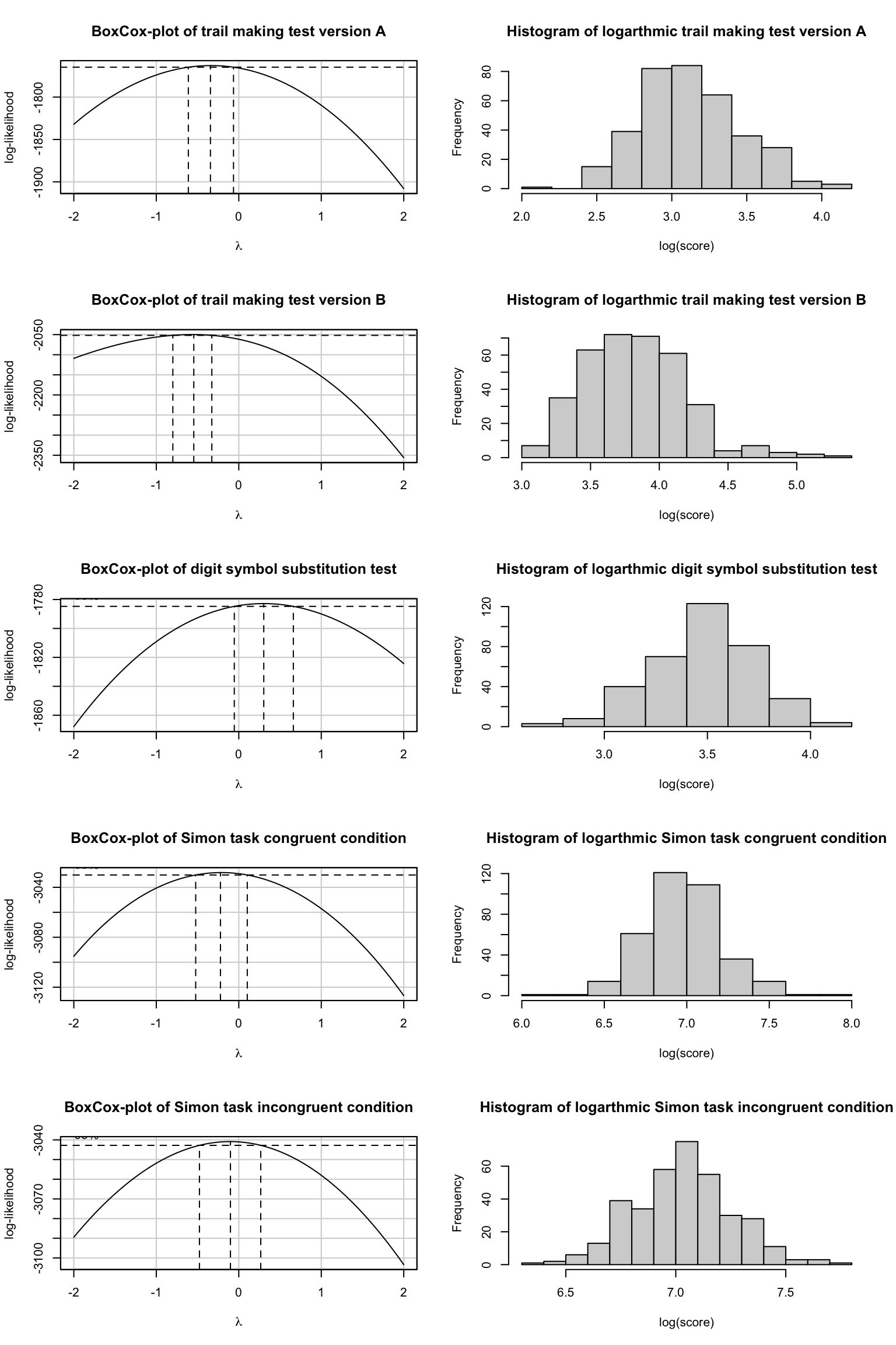
A Box-Cox distribution analysis (Box & Cox, 1964) suggested logarithmic transformations for all executive function tests to obtain normally distributed model residuals (see Figure 8.1). Accordingly, lag transformed means and standard deviations were used for z-transformation (see Table 8.2). Further, the z-transformed scores for the trail making test and Simon task were reversed, so positive improvements of z-values indicate and improvement in time to completion or reaction time.

data.frame(Test=c("TMTa (s)","TMTb (s)","DSST (n)","SC (ms)","SI (ms)"),
           mean=c("3.12","3.83","3.47","6.97","7.03"),
           sd=c("0.328","0.370","0.244","0.228","0.223")) |> 
  flextable() |> 
  autofit() |> 
  align(j=2:3, align = "right") |> 
  add_footer_row(values = c("TMTa = trail making test verion A, TMTb = trail making test version B, DSST = digit symbol substitution test, SC = Simon task congruent condition, SI = Simon task incongruent condition"), colwidths  = 3)

Table 8.2: Mean and standard deviation of executive function log-scores

cog <- as_tibble(tx) |>
  select(Child = "id",contains("dsst"),
         contains("tmt") & ends_with("Time"),
         contains("simon_m.rt")) |>
  mutate(t0_cog_dsst_dsst.score=t0_cog_dsst_num-t0_cog_dsst_err,
         t1_cog_dsst_dsst.score=t1_cog_dsst_num-t1_cog_dsst_err,
         t2_cog_dsst_dsst.score=t2_cog_dsst_num-t2_cog_dsst_err,
         t3_cog_dsst_dsst.score=t3_cog_dsst_num-t3_cog_dsst_err,
         t6_cog_dsst_dsst.score=t6_cog_dsst_num-t6_cog_dsst_err,
         t8_cog_dsst_dsst.score=t8_cog_dsst_num-t8_cog_dsst_err) |>
  select(-contains("num")&-contains("err")) |>
  pivot_longer(2:31, names_to = c("Time","type","domain", "Test"),
               names_sep = "_", values_to = "Score") |> 
  select(-domain, -type) |> 
  mutate(across(where(is.character), as.factor),
        Test = fct_recode(Test, TMTa = "a.time", TMTb = "b.time", DSST = "dsst.score",
                           SC = "m.rt.con", SI = "m.rt.incon"),
        Test = fct_relevel(Test, "TMTa", "TMTb", "DSST", "SC", "SI"),
        zScore = case_when(Test == "TMTa" ~ -(log(Score) - 3.12)/.328,
                           Test == "TMTb" ~ -(log(Score) - 3.83)/.370,
                           Test == "DSST" ~ (log(Score) - 3.47)/.244,
                           Test == "SC" ~ -(log(Score) - 6.97)/.228,
                           Test == "SI" ~ -(log(Score) - 7.03)/.223))

save(cog, file="data/cog.rda")

par(mfrow=c(5,2))
car::boxCox(lm(Score ~ 1, data = cog[which(cog$Test=="TMTa"),]), main = "BoxCox-plot of trail making test version A") 
hist(log(cog[which(cog$Test=="TMTa"),]$Score), main = "Histogram of logarthmic trail making test version A", xlab = "log(score)")
car::boxCox(lm(Score ~ 1, data = cog[which(cog$Test=="TMTb"),]), main = "BoxCox-plot of trail making test version B") 
hist(log(cog[which(cog$Test=="TMTb"),]$Score), main = "Histogram of logarthmic trail making test version B", xlab = "log(score)")
car::boxCox(lm(Score ~ 1, data = cog[which(cog$Test=="DSST"),]), main = "BoxCox-plot of digit symbol substitution test") 
hist(log(cog[which(cog$Test=="DSST"),]$Score), main = "Histogram of logarthmic digit symbol substitution test", xlab = "log(score)")
car::boxCox(lm(Score ~ 1, data = cog[which(cog$Test=="SC"),]), main = "BoxCox-plot of Simon task congruent condition") 
hist(log(cog[which(cog$Test=="SC"),]$Score), main = "Histogram of logarthmic Simon task congruent condition", xlab = "log(score)")
car::boxCox(lm(Score ~ 1, data = cog[which(cog$Test=="SI"),]), main = "BoxCox-plot of Simon task incongruent condition") 
hist(log(cog[which(cog$Test=="SI"),]$Score), main = "Histogram of logarthmic Simon task incongruent condition", xlab = "log(score)")

Figure 8.1: Box-Cox distribution and histograms of executive function tests

8.2 Supplementary Material Chapter 2

8.2.1 Body mass index analysis for t1 and t3 populations

data_t1 <- left_join(info, anthro) |>
  select(Child, school, Group, gender, Time, bmi) |> 
  subset(Time %in% c("t0","t1")) |> 
  mutate(across(where(is.character), as.factor)) 
  
contrasts(data_t1$Group) <- MASS::contr.sdif(2)
contrasts(data_t1$gender)  <- MASS::contr.sdif(2)
contrasts(data_t1$Time) <- MASS::contr.sdif(2)

m_bmi_t1 <- lmer(bmi ~ 1 + Group*gender*Time + (1 | Child) + (1 | school), data=data_t1, REML=FALSE,
              control=lmerControl(calc.derivs=FALSE))

tab2 <- tab_model(m_bmi_t1, digits=2, digits.re=2, show.se=TRUE, show.stat=TRUE, show.ci=FALSE,CSS = css_theme("cells"),
          pred.labels = c("Grand mean", "Group2-1", "gender2-1", "Time2-1", "Group2-1 * gender2-1", "Group2-1 * Time2-1", "gender2-1* Time2-1", "Group2-1 * gender2-1 * Time2-1"))

tab_to_flex(tab2,"")

Table 8.3: Group x gender x Time interactions for body mass index for the first intervention period (i.e., t0 to t1)

data_t3 <- left_join(info, anthro) |>
  select(Child, school, Group, gender, Time, bmi) |> 
  subset(Time %in% c("t0","t1","t2","t3")) |> 
  mutate(across(where(is.character), as.factor)) 
  
contrasts(data_t3$Group) <- MASS::contr.sdif(2)
contrasts(data_t3$gender)  <- MASS::contr.sdif(2)
contrasts(data_t3$Time) <- MASS::contr.sdif(4)

m_bmi_t3 <- lmer(bmi ~ 1 + Group*gender*Time + (1 | Child) + (1 | school), data=data_t3, REML=FALSE,
              control=lmerControl(calc.derivs=FALSE))

tab3 <- tab_model(m_bmi_t3, digits=2, digits.re=2, show.se=TRUE, show.stat=TRUE, show.ci=FALSE,CSS = css_theme("cells"),
                  pred.labels = c("Grand mean", "Group2-1", "gender2-1", "Time2-1", "Time3-2", "Time4-3", "Group2-1 * gender2-1", "Group2-1 * Time2-1", "Group2-1 * Time3-2", "Group2-1 * Time4-3", "gender2-1 * Time2-1", "gender2-1 * Time3-2", "gender2-1 * Time4-3", "Group2-1 * gender2-1 * Time2-1", "Group2-1 * gender2-1 * Time3-2", "Group2-1 * gender2-1 * Time4-3"))

tab_to_flex(tab3,"")

Table 8.4: Group x gender x Time interactions for body mass index for both intervention periods (i.e., t0 to t3)

8.3 Supplementary Material Chapter 3

8.3.1 INT M1: physical fitness

8.3.1.1 Model fitting

data_m1 <- left_join(info, anthro) |>
  left_join(ages) |>
  select(Child, bp, Group, gender, Time, bmi, age) |>
  filter(!(Child %in% c("SMART06", "SMART23", "SMART58", "SMART68")),
         Time %in% c("t0","t1"))|> 
  mutate(across(where(is.character), \(x) as.factor(x))) |> 
  arrange(Child, Time) |> 
  fill(bmi)

Joining with `by = join_by(Child, Time)`
Joining with `by = join_by(Child, Time)`

data_m1_emo <- data_m1 |>
  left_join(emo) |> 
  filter(!is.na(zScore) & Test %in% c("Run", "Star_r", "S20_r", "SLJ")) |>
  mutate(a1=age - 9.3,
         bmi_c=ifelse(gender=="girl", bmi-17.9,bmi-19.8),
         Test=droplevels(Test),
         Time=droplevels(Time))

Joining with `by = join_by(Child, Time)`

contrasts(data_m1_emo$Test)  <- MASS::contr.sdif(4)
contrasts(data_m1_emo$Time)  <- MASS::contr.sdif(2)
contrasts(data_m1_emo$Group) <- MASS::contr.sdif(2)
contrasts(data_m1_emo$gender)   <- MASS::contr.sdif(2)
contrasts(data_m1_emo$bp)   <- MASS::contr.sdif(2)

m1.1_emo <- lmer(zScore ~ 0 + Test + (1 | Child), data = data_m1_emo, REML = FALSE, control = lmerControl(calc.derivs = FALSE))
m1.2_emo      <- update(m1.1_emo, . ~ .  -Test + Test/(Group * Time))
m1.3_emo_abp  <- update(m1.2_emo, . ~ .           + a1 + bmi_c + bp)
m1.3_emo_gbp  <- update(m1.2_emo, . ~ .  + gender      + bmi_c + bp)
m1.3_emo_gap  <- update(m1.2_emo, . ~ .  + gender + a1         + bp)
m1.3_emo_gab  <- update(m1.2_emo, . ~ .  + gender + a1 + bmi_c     )
m1.4_emo_all  <- update(m1.2_emo, . ~ .  + gender + a1 + bmi_c + bp)

Warning: There was 1 warning in `mutate()`.
ℹ In argument: `across(where(is.numeric), round, 3)`.
Caused by warning:
! The `...` argument of `across()` is deprecated as of dplyr 1.1.0.
Supply arguments directly to `.fns` through an anonymous function instead.

  # Previously
  across(a:b, mean, na.rm = TRUE)

  # Now
  across(a:b, \(x) mean(x, na.rm = TRUE))

LRT indicated that body mass index (BMI) improves the model’s fit, while age, gender, and Berlin proximity can be dropped.

m1.5_emo_bmi <- update(m1.1_emo, . ~ . - Test + Test/(Group * Time) + bmi_c)
m1.6_emo_bmi <- update(m1.1_emo, . ~ . - Test + Test/(Group * Time + bmi_c))
m1.7_emo_bmi <- update(m1.1_emo, . ~ . - Test + Test/((Group + Time + bmi_c)^2))

LRT further showed that including BMI nested within Test without interactions improves the models fit. Accordingly, m1.6_emo_bmi was reported in Section 3.3.1.1.

8.3.1.2 Means and standard deviations of model variables

`summarise()` has grouped output by 'Time'. You can override using the
`.groups` argument.

8.3.2 INT M1: executive function

8.3.2.1 Model fitting

data_m1_cog <- data_m1 |>
  left_join(cog) |> 
  filter(!is.na(zScore)) |>
  mutate(a1=age - 9.3,
         bmi_c=ifelse(gender=="girl", bmi-17.9,bmi-19.8),
         Test=droplevels(Test),
         Time=droplevels(Time))

contrasts(data_m1_cog$Test) <- MASS::contr.sdif(5)
contrasts(data_m1_cog$Time)  <- MASS::contr.sdif(2)
contrasts(data_m1_cog$Group) <- MASS::contr.sdif(2)
contrasts(data_m1_cog$gender)   <- MASS::contr.sdif(2)
contrasts(data_m1_cog$bp)   <- MASS::contr.sdif(2)

m1.1_cog <- lmer(zScore ~ 0 + Test + (1 | Child), data = data_m1_cog, REML = FALSE, control = lmerControl(calc.derivs = FALSE))
m1.2_cog     <- update(m1.1_cog, . ~ .  -Test + Test/(Group * Time))
m1.3_cog_abp <- update(m1.2_cog, . ~ .           + a1 + bmi_c + bp)
m1.3_cog_gbp <- update(m1.2_cog, . ~ .  + gender      + bmi_c + bp)
m1.3_cog_gap <- update(m1.2_cog, . ~ .  + gender + a1         + bp)
m1.3_cog_gab <- update(m1.2_cog, . ~ .  + gender + a1 + bmi_c     )
m1.4_cog_all <- update(m1.2_cog, . ~ .  + gender + a1 + bmi_c + bp)

LRT indicated that gender improves the model’s fit, while age, BMI, and Berlin proximity can be dropped.

m1.5_cog_gender <- update(m1.1_cog, . ~ . - Test + Test/(Group * Time) + gender)
m1.6_cog_gender <- update(m1.1_cog, . ~ . - Test + Test/(Group * Time + gender))
m1.7_cog_gender <- update(m1.1_cog, . ~ . - Test + Test/((Group + Time + gender)^2))

LRT further showed that gender added as a fixed factor not nested within Test improves the models fit. Accordingly, m1.5_cog_bmi was reported in Section 3.3.2.1.

8.3.2.2 Means and standard deviations of model variables

`summarise()` has grouped output by 'Time'. You can override using the
`.groups` argument.

8.3.3 INT M2: physical fitness

8.3.3.1 Model fitting

data_m2 <- left_join(info, anthro) |>
  left_join(ages) |>
  select(Child, bp, Group, gender, Time, bmi, age) |>
  filter(!(Child %in% c("SMART01", "SMART06", "SMART12", "SMART19", "SMART23", 
                     "SMART39", "SMART58", "SMART63", "SMART68", "SMART75" )),
         Time %in% c("t0","t1","t2","t3"))|> 
  mutate(Group_pooled = case_when(Group== "INT-CON" & Time %in% c("t0", "t1") ~ "INT",
                                  Group== "INT-CON" & Time %in% c("t2", "t3") ~ "CON",
                                  Group== "CON-INT" & Time %in% c("t0", "t1") ~ "CON",
                                  Group== "CON-INT" & Time %in% c("t2", "t3") ~ "INT"),
         Time_pooled = case_when(Time %in% c("t0", "t2") ~ "pre",
                           Time %in% c("t1", "t3") ~ "post"),
         Time_pooled=factor(Time_pooled, levels = c("pre","post")),
         across(where(is.character), as.factor)) |> 
  arrange(Child, Time) |> 
  fill(bmi)

Joining with `by = join_by(Child, Time)`
Joining with `by = join_by(Child, Time)`

data_m2_emo <- data_m2 |>
  left_join(emo) |> 
  filter(!is.na(zScore) & Test %in% c("Run", "Star_r", "S20_r", "SLJ")) |>
  mutate(a1=age - 9.6,
         bmi_c=ifelse(gender=="girl", bmi-18.5,bmi-19.9),
         Test=droplevels(Test))

Joining with `by = join_by(Child, Time)`

contrasts(data_m2_emo$Time_pooled)  <- MASS::contr.sdif(2)
contrasts(data_m2_emo$Group_pooled) <- MASS::contr.sdif(2)
contrasts(data_m2_emo$gender)   <- MASS::contr.sdif(2)
contrasts(data_m2_emo$bp)   <- MASS::contr.sdif(2)
contrasts(data_m2_emo$Test)  <- MASS::contr.sdif(4)

m2.1_emo <- lmer(zScore ~ 0 + Test + (1 | Child), data = data_m2_emo, REML = FALSE, control = lmerControl(calc.derivs = FALSE))
m2.2_emo     <- update(m2.1_emo, . ~ .  -Test + Test/(Group_pooled * Time_pooled))
m2.3_emo_abp <- update(m2.2_emo, . ~ .           + a1 + bmi_c + bp)
m2.3_emo_gbp <- update(m2.2_emo, . ~ .  + gender      + bmi_c + bp)
m2.3_emo_gap <- update(m2.2_emo, . ~ .  + gender + a1         + bp)
m2.3_emo_gab <- update(m2.2_emo, . ~ .  + gender + a1 + bmi_c     )
m2.4_emo_all <- update(m2.2_emo, . ~ .  + gender + a1 + bmi_c + bp)

LRT indicated that BMI improves the model’s fit, while age, gender, and Berlin proximity can be dropped.

m2.5_emo_bmi <- update(m2.1_emo, . ~ . - Test + Test/(Group_pooled * Time_pooled) + bmi_c)
m2.6_emo_bmi <- update(m2.1_emo, . ~ . - Test + Test/(Group_pooled * Time_pooled + bmi_c))
m2.7_emo_bmi <- update(m2.1_emo, . ~ . - Test + Test/((Group_pooled + Time_pooled + bmi_c)^2))

LRT further showed that BMI added as a fixed factor nested within Test without interactions improves the models fit. Accordingly, m2.6_emo_bmi was reported in Section 3.4.1.1.

8.3.3.2 Means and standard deviations of model variables

`summarise()` has grouped output by 'Time_pooled'. You can override using the
`.groups` argument.

8.3.4 INT M2: executive function

8.3.4.1 Model fitting

data_m2_cog <- data_m2 |>
  left_join(cog) |> 
  filter(!is.na(zScore)) |>
  mutate(a1=age - 9.6,
         bmi_c=ifelse(gender=="girl", bmi-18.5,bmi-19.9),
         Test=droplevels(Test))

Joining with `by = join_by(Child, Time)`

contrasts(data_m2_cog$Time_pooled)  <- MASS::contr.sdif(2)
contrasts(data_m2_cog$Group_pooled) <- MASS::contr.sdif(2)
contrasts(data_m2_cog$gender)   <- MASS::contr.sdif(2)
contrasts(data_m2_cog$bp)   <- MASS::contr.sdif(2)
contrasts(data_m2_cog$Test)  <- MASS::contr.sdif(5)

m2.1_cog <- lmer(zScore ~ 0 + Test + (1 | Child), data = data_m2_cog, REML = FALSE, control = lmerControl(calc.derivs = FALSE))
m2.2_cog     <- update(m2.1_cog, . ~ .  -Test + Test/(Group_pooled * Time_pooled))
m2.3_cog_abp <- update(m2.2_cog, . ~ .           + a1 + bmi_c + bp)
m2.3_cog_gbp <- update(m2.2_cog, . ~ .  + gender      + bmi_c + bp)
m2.3_cog_gap <- update(m2.2_cog, . ~ .  + gender + a1         + bp)
m2.3_cog_gab <- update(m2.2_cog, . ~ .  + gender + a1 + bmi_c     )
m2.4_cog_all <- update(m2.2_cog, . ~ .  + gender + a1 + bmi_c + bp)

LRT indicated that age improves the model’s fit, while BMI, gender, and Berlin proximity can be dropped.

m2.5_cog_gender <- update(m2.1_cog, . ~ . - Test + Test/(Group_pooled * Time_pooled) + a1)
m2.6_cog_gender <- update(m2.1_cog, . ~ . - Test + Test/(Group_pooled * Time_pooled + a1))
m2.7_cog_gender <- update(m2.1_cog, . ~ . - Test + Test/((Group_pooled + Time_pooled + a1)^2))

LRT further showed that age added as a fixed factor not nested within Test improves the models fit. Accordingly, m2.5_cog_bmi was reported in Section 3.4.2.1.

8.3.4.2 Means and standard deviations of model variables

`summarise()` has grouped output by 'Time_pooled'. You can override using the
`.groups` argument.

8.3.5 INT M3: physical fitness

8.3.5.1 Model fitting

data_m3 <- left_join(info, anthro) |>
  left_join(ages) |>
  select(Child, bp, Group, gender, Time, bmi, age) |>
  filter(!(Child%in% c(
"SMART01", "SMART03", "SMART04", "SMART05", "SMART06", "SMART07", "SMART08", "SMART09", "SMART10", "SMART12", "SMART13", "SMART14", "SMART16", "SMART19", "SMART21", "SMART22", "SMART23", "SMART28", "SMART31", "SMART33", "SMART37", "SMART38", "SMART39", "SMART40", "SMART43", "SMART52", "SMART56", "SMART57", "SMART58", "SMART61", "SMART63", "SMART64", "SMART68", "SMART69", "SMART70", "SMART71", "SMART72", "SMART75", "SMART76"  )),
         Time %in% c("t0","t1","t2","t3","t6","t8")) |> 
  mutate(bp=ifelse(bp=="01","09",bp),
         across(where(is.character), as.factor)) |>
  arrange(Child, Time) |> 
  fill(bmi)

Joining with `by = join_by(Child, Time)`
Joining with `by = join_by(Child, Time)`

data_m3_emo <- data_m3 |>
  left_join(emo) |> 
  filter(!is.na(zScore) & Test %in% c("Run", "Star_r", "S20_r", "SLJ")) |>
  mutate(a1=age - 10,
         bmi_c=ifelse(gender=="girl", bmi-19.7,bmi-20.4),
         Test=droplevels(Test))

Joining with `by = join_by(Child, Time)`

contrasts(data_m3_emo$Test)  <- MASS::contr.sdif(4)
contrasts(data_m3_emo$Time)  <- MASS::contr.sdif(6)
contrasts(data_m3_emo$Group) <- MASS::contr.sdif(2)
contrasts(data_m3_emo$gender)   <- MASS::contr.sdif(2)
contrasts(data_m3_emo$bp)   <- MASS::contr.sdif(2)

m3.1_emo <- lmer(zScore ~ 0 + Test + (1 | Child), data = data_m3_emo, REML = FALSE, control = lmerControl(calc.derivs = FALSE))
m3.2_emo     <- update(m3.1_emo, . ~ .  -Test + Test/(Group * Time))
m3.3_emo_abp <- update(m3.2_emo, . ~ .           + a1 + bmi_c + bp)
m3.3_emo_gbp <- update(m3.2_emo, . ~ .  + gender      + bmi_c + bp)
m3.3_emo_gap <- update(m3.2_emo, . ~ .  + gender + a1         + bp)
m3.3_emo_gab <- update(m3.2_emo, . ~ .  + gender + a1 + bmi_c     )
m3.4_emo_all <- update(m3.2_emo, . ~ .  + gender + a1 + bmi_c + bp)

LRT indicated that BMI and Berlin proximity improves the model’s fit, while age and gender can be dropped.

m3.5_emo_bmi <- update(m3.1_emo, . ~ . - Test + Test/(Group * Time) + bmi_c)
m3.6_emo_bmi <- update(m3.1_emo, . ~ . - Test + Test/(Group * Time + bmi_c))
m3.7_emo_bmi <- update(m3.1_emo, . ~ . - Test + Test/((Group + Time + bmi_c)^2))
m3.5_emo_bp <- update(m3.1_emo, . ~ . - Test + Test/(Group * Time) + bp)
m3.6_emo_bp <- update(m3.1_emo, . ~ . - Test + Test/(Group * Time + bp))
m3.7_emo_bp <- update(m3.1_emo, . ~ . - Test + Test/((Group + Time + bp)^2))

fixed-effect model matrix is rank deficient so dropping 4 columns / coefficients

LRT indicated that BMI and Berlin proximity added in the fixed structure nested within Test improves the model’s fit.

m3.6_emo_bmibp <- update(m3.1_emo, . ~ . - Test + Test/(Group * Time + bmi_c + bp))
m3.6_emo_bmibp2 <- update(m3.1_emo, . ~ . - Test + Test/(Group * Time + bmi_c * bp))

LRT further indicated that BMI and Berlin proximity both added to the fixed structure nested within Test without interactions improves the model’s fit. Accordingly, m3.6_emo_bmibp was reported in Section 3.5.1.1.

8.3.5.2 Means and standard deviations of model variables

`summarise()` has grouped output by 'Time'. You can override using the
`.groups` argument.

8.3.6 INT M3: executive function

8.3.6.1 Model fitting

data_m3_cog <- data_m3 |>
  left_join(cog) |> 
  filter(!is.na(zScore)) |>
  mutate(a1=age - 10,
         bmi_c=ifelse(gender=="girl", bmi-19.7,bmi-20.4),
         Test=droplevels(Test))

Joining with `by = join_by(Child, Time)`

contrasts(data_m3_cog$Time)  <- MASS::contr.sdif(6)
contrasts(data_m3_cog$Group) <- MASS::contr.sdif(2)
contrasts(data_m3_cog$bp) <- MASS::contr.sdif(2)
contrasts(data_m3_cog$gender)   <- MASS::contr.sdif(2)
contrasts(data_m3_cog$Test)  <- MASS::contr.sdif(5)

m3.1_cog <- lmer(zScore ~ 0 + Test + (1 | Child), data = data_m3_cog, REML = FALSE, control = lmerControl(calc.derivs = FALSE))
m3.2_cog     <- update(m3.1_cog, . ~ .  -Test + Test/(Group * Time))
m3.3_cog_abp <- update(m3.2_cog, . ~ .           + a1 + bmi_c + bp)
m3.3_cog_gbp <- update(m3.2_cog, . ~ .  + gender      + bmi_c + bp)
m3.3_cog_gap <- update(m3.2_cog, . ~ .  + gender + a1         + bp)
m3.3_cog_gab <- update(m3.2_cog, . ~ .  + gender + a1 + bmi_c     )
m3.4_cog_all <- update(m3.2_cog, . ~ .  + gender + a1 + bmi_c + bp)

LRT indicated that including BMI, Berlin proximity, age, and gender in the fixed factors do not improve the model’s fit. Accordingly, all covariates were dropped and m3.2_cog was reported in Section 3.5.2.1.

8.3.6.2 Means and standard deviations of model variables

`summarise()` has grouped output by 'Time'. You can override using the
`.groups` argument.

8.4 Supplementary Material Chapter 4

data_5 <- left_join(info, ages) |>
  left_join(anthro) |> 
  left_join(emo) |> 
  mutate(across(where(is.character), as.factor),
         muscle_p=muscle/mass*100,
         fat_p=fat,
         fat=(mass*(fat_p/100)),
         w_mf=muscle + fat,
         bmi=height/(mass^2),
         a1=age-9.9,
         gender=factor(gender, levels = c("girl","boy"))) |> 
  select(Child, Time, a1, gender, Test, Score, zScore, mass, height, muscle, muscle_p, fat, fat_p, w_mf, lean) |> 
  subset(is.na(zScore)==FALSE)|> 
  arrange(Child, Time) |> 
  fill(mass:lean)

Joining with `by = join_by(Child, Time)`
Joining with `by = join_by(Child, Time)`
Joining with `by = join_by(Child, Time)`

8.4.1 Correlation of InBody parameters

data_5 |> 
  select(height,mass,fat, fat_p,muscle, muscle_p, w_mf, lean) |> 
  PerformanceAnalytics::chart.Correlation(histogram = "TRUE", method = "pearson") 

Warning in par(usr): argument 1 does not name a graphical parameter

Warning in par(usr): argument 1 does not name a graphical parameter

Warning in par(usr): argument 1 does not name a graphical parameter

Warning in par(usr): argument 1 does not name a graphical parameter

Warning in par(usr): argument 1 does not name a graphical parameter

Warning in par(usr): argument 1 does not name a graphical parameter

Warning in par(usr): argument 1 does not name a graphical parameter

Warning in par(usr): argument 1 does not name a graphical parameter

Warning in par(usr): argument 1 does not name a graphical parameter

Warning in par(usr): argument 1 does not name a graphical parameter

Warning in par(usr): argument 1 does not name a graphical parameter

Warning in par(usr): argument 1 does not name a graphical parameter

Warning in par(usr): argument 1 does not name a graphical parameter

Warning in par(usr): argument 1 does not name a graphical parameter

Warning in par(usr): argument 1 does not name a graphical parameter

Warning in par(usr): argument 1 does not name a graphical parameter

Warning in par(usr): argument 1 does not name a graphical parameter

Warning in par(usr): argument 1 does not name a graphical parameter

Warning in par(usr): argument 1 does not name a graphical parameter

Warning in par(usr): argument 1 does not name a graphical parameter

Warning in par(usr): argument 1 does not name a graphical parameter

Warning in par(usr): argument 1 does not name a graphical parameter

Warning in par(usr): argument 1 does not name a graphical parameter

Warning in par(usr): argument 1 does not name a graphical parameter

Warning in par(usr): argument 1 does not name a graphical parameter

Warning in par(usr): argument 1 does not name a graphical parameter

Warning in par(usr): argument 1 does not name a graphical parameter

Warning in par(usr): argument 1 does not name a graphical parameter

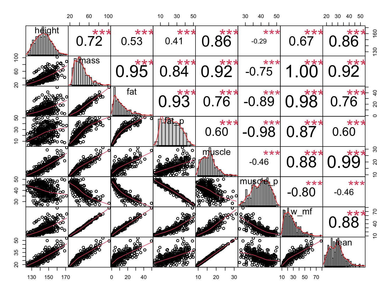
Correlations for anthropometric parameters assessed using the InBody; height = body height [cm], mass = body mass [kg], fat = body fat mass [kg], fat_p = body fat percent [%], muscle = body muscle mass [kg], muscle_p = body muscle mass percent [%], w_mf = sum of muscle mass and fat mass [kg], lean = body lean mass

8.4.2 Model selection

dat_5 <- data_5 |> 
  subset(Test %in% c("Run", "Star_r", "S20_r", "SLJ", "BPT")) |> 
  mutate(m=mass-40.96,
         m2=m*m,
         h=height-143.51,
         h2=h*h,
         Test=factor(Test, levels = c("Run", "Star_r", "S20_r", "SLJ", "BPT"))) |> 
  select(Child, a1, Test, zScore, m, m2, h, h2)

contrasts(dat_5$Test)   <- MASS::contr.sdif(5)

m1     <- lmer(zScore ~ 0 + a1 + (1 + a1 | Child), data = dat_5, REML = FALSE, control = lmerControl(calc.derivs = FALSE))
m1_0   <- update(m1, . ~ + Test +         .)
m1_m   <- update(m1, . ~ + Test/(    m) + .)
m1_h   <- update(m1, . ~ + Test/(h    ) + .)
m1_hm  <- update(m1, . ~ + Test/(h + m) + .)

Including body mass and height into the model, nested within Test, improve the fit.

m2_h2    <- update(m1, . ~ + Test/(m + h      + h2)  + .)
m2_m2    <- update(m1, . ~ + Test/(m + h + m2     )  + .)
m2_h2m2  <- update(m1, . ~ + Test/(m + h + m2 + h2)  + .)

LRT revealed only significant quadratic effects for body mass improves models fit.

m3_hm1  <- update(m1, . ~ + Test/(h * m +     m2) + .)
m3_hm2  <- update(m1, . ~ + Test/(h * m + h * m2) + .)

Warning: Some predictor variables are on very different scales: consider
rescaling

Second-order interactions showed significant improvements in models fitted for interactions of body size with linear but not quadratic trends in body mass. Accordingly, m3_hm1 was reported in Section 4.2.

8.4.3 Means and standard deviations of model variables

8.5 Supplementary Material Chapter 5

load(file="data/info.rda")
load(file="data/ages.rda")
load(file="data/emo.rda")

data_4 <- info |>
  left_join(ages) |>
  left_join(emo) |>
  mutate(across(where(is.character), as.factor),
         gender=factor(gender, levels = c("girl","boy")),
         a1=age-9.9,
         m1=m_mirwald+2.25,
         m2=m_moore+2.34,
         m1pc1=(scale(age)+scale(m_mirwald))/2,
         m1pc2=(scale(age)-scale(m_mirwald)),
         m2pc1=(scale(age)+scale(m_moore))/2,
         m2pc2=(scale(age)-scale(m_moore))) |> 
  select(Child, gender, Time, Test, zScore, Score, a1, m1, m2, m1pc1, m1pc2, m2pc1, m2pc2) |> 
  fill(a1:m2pc2)

cbPalette <- c( "#0072B2", "#D55E00", "#009E73", "#CC79A7",
                "#F0E442", "#56B4E9", "#999999", "#E69F00")

8.5.1 Correlation age, maturity, and their principal components

data_4 |> 
  select(a1:m2pc2) |> 
  PerformanceAnalytics::chart.Correlation(histogram = "TRUE", method = "pearson") 

Warning in par(usr): argument 1 does not name a graphical parameter

Warning in par(usr): argument 1 does not name a graphical parameter

Warning in par(usr): argument 1 does not name a graphical parameter

Warning in par(usr): argument 1 does not name a graphical parameter

Warning in par(usr): argument 1 does not name a graphical parameter

Warning in par(usr): argument 1 does not name a graphical parameter

Warning in par(usr): argument 1 does not name a graphical parameter

Warning in par(usr): argument 1 does not name a graphical parameter

Warning in par(usr): argument 1 does not name a graphical parameter

Warning in par(usr): argument 1 does not name a graphical parameter

Warning in par(usr): argument 1 does not name a graphical parameter

Warning in par(usr): argument 1 does not name a graphical parameter

Warning in par(usr): argument 1 does not name a graphical parameter

Warning in par(usr): argument 1 does not name a graphical parameter

Warning in par(usr): argument 1 does not name a graphical parameter

Warning in par(usr): argument 1 does not name a graphical parameter

Warning in par(usr): argument 1 does not name a graphical parameter

Warning in par(usr): argument 1 does not name a graphical parameter

Warning in par(usr): argument 1 does not name a graphical parameter

Warning in par(usr): argument 1 does not name a graphical parameter

Warning in par(usr): argument 1 does not name a graphical parameter

Correlations for age-related parameters; a1 = age centered at 0 [years], m1 = maturity offset centered at 0 (Mirwald) [years], m2 = maturity offset centered at 0 (Moore) [years], m1pc1 = first principal component of age and maturity (Mirwald) [z-score], m1pc2 = second principal component of age and maturity (Mirwald) [z-score], m2pc1 = first principal component of age and maturity (Moore) [z-score], m2pc2 = second principal component of age and maturity (Moore) [z-score]

8.5.2 Model 1: Effect of maturity offset according to Mirwald, age, and gender on physical fitness

8.5.2.1 Model selection

dat_41 <- data_4 |> 
  subset(Test %in% c("Run", "Star_r", "S20_r", "SLJ")) |>
  select(Child, Time, gender, a1, m1, m1pc1, m1pc2, Test, zScore) |> 
  mutate(Test=factor(Test, levels = c("Run", "Star_r", "S20_r", "SLJ"))) |> 
  na.omit()

contrasts(dat_41$Time)   <- MASS::contr.sdif(6)
contrasts(dat_41$Test)   <- MASS::contr.sdif(4)
contrasts(dat_41$gender) <- MASS::contr.sdif(2)

m1  <- lmer(zScore ~ 0 + (1 | Child), data = dat_41, REML = FALSE, control = lmerControl(calc.derivs = FALSE))
m2_all <- update(m1, . ~ . + Test/(m1pc1 + m1pc2 + gender))
m2_p1  <- update(m1, . ~ . + Test/(        m1pc2 + gender))
m2_p2  <- update(m1, . ~ . + Test/(m1pc1         + gender))
m2_ge  <- update(m1, . ~ . + Test/(m1pc1 + m1pc2         ))

Table 8.5: LRT 1 of fixed effects in Model 1

LRTs indicate that both principal components and gender improve the models fit.

m311 <- update(m1, . ~ . + Test/(gender/(m1pc1) + m1pc2))
m312 <- update(m1, . ~ . + Test/(gender/(m1pc2) + m1pc1))
m32  <- update(m1, . ~ . + Test/(gender/(m1pc1 + m1pc2)))
m33  <- update(m1, . ~ . + Test/(gender/(m1pc1 * m1pc2)))

Table 8.6: LRT 2 of fixed effects in Model 1

LRTs reveal a significance third order interaction, however the model is very likely to be overparametrise according to AIC and BIC.

m3_p1 <- update(m2_all, . ~ . - (1 | Child) + (1 + m1pc1         | Child))
m3_p2 <- update(m2_all, . ~ . - (1 | Child) + (1         + m1pc2 | Child))
m3    <- update(m2_all, . ~ . - (1 | Child) + (1 + m1pc1 + m1pc2 | Child))

Table 8.7: LRT 3 of fixed effects in Model 1

Both principal components entered into the random effect structure of Child did significantly improve the fit of the model. Accordingly, m3 will be reported in Section 5.3.

8.5.3 Model 2: Effect of maturity offset according to Moore, age, and gender on physical fitness

8.5.3.1 Model selection

dat_42 <- data_4 |> 
  subset(Test %in% c("Run", "Star_r", "S20_r", "SLJ")) |>
  select(Child, gender, m2pc1, m2pc2, Test, zScore) |> 
  mutate(Test=factor(Test, levels = c("Run", "Star_r", "S20_r", "SLJ"))) |> 
  na.omit()

contrasts(dat_42$Test)   <- MASS::contr.sdif(4)
contrasts(dat_42$gender) <- MASS::contr.sdif(2)

m4     <- lmer(zScore ~ 0 + (1 | Child), data = dat_42, REML = FALSE, control = lmerControl(calc.derivs = FALSE))
m5_all <- update(m4, . ~ . + Test/(m2pc1 + m2pc2 + gender))
m5_p1  <- update(m4, . ~ . + Test/(        m2pc2 + gender))
m5_p2  <- update(m4, . ~ . + Test/(m2pc1         + gender))
m5_ge  <- update(m4, . ~ . + Test/(m2pc1 + m2pc2         ))

Table 8.8: LRT 1 of fixed effects in Model 2

LRTs indicate that both principal components and gender improve the models fit.

m511 <- update(m4, . ~ . + Test/(gender/(m2pc1) + m2pc2))
m512 <- update(m4, . ~ . + Test/(gender/(m2pc2) + m2pc1))
m52  <- update(m4, . ~ . + Test/(gender/(m2pc1 + m2pc2)))
m53  <- update(m4, . ~ . + Test/(gender/(m2pc1 * m2pc2)))

Table 8.9: LRT 2 of fixed effects in Model 2

LRTs reveal a significance third order interaction, however the model is very likely to be overparametrise according to AIC and BIC.

m6_p1 <- update(m5_all, . ~ . - (1 | Child) + (1 + m2pc1         | Child))
m6_p2 <- update(m5_all, . ~ . - (1 | Child) + (1         + m2pc2 | Child))
m6    <- update(m5_all, . ~ . - (1 | Child) + (1 + m2pc1 + m2pc2 | Child))

Table 8.10: LRT 3 of fixed effects in Model 2

Both principal components entered into the random effect structure of Child did significantly improve the fit of the model. Accordingly, m6 will be reported in Section 5.4.

8.5.4 Means and standard deviations of model variables

Joining with `by = join_by(Child, Time)`
Joining with `by = join_by(Child, Time)`

Box, G. E. P., & Cox, D. R. (1964). An analysis of transformations. Journal of the Royal Statistical Society: Series B (Methodological), 26. https://doi.org/10.1111/j.2517-6161.1964.tb00553.x

Fühner, T., Granacher, U., Golle, K., & Kliegl, R. (2021). Age and sex effects in physical fitness components of 108,295 third graders including 515 primary schools and 9 cohorts. Scientific Reports, 11. https://doi.org/10.1038/s41598-021-97000-4

Fühner, T., Granacher, U., Golle, K., & Kliegl, R. (2022). Effect of timing of school enrollment on physical fitness in third graders. Nature - Scientific Reports, 12.

Mirwald, R. L., Baxter-Jones, A. D. G., Bailey, D. A., & Beunen, G. P. (2002). An assessment of maturity from anthropometric measurements. Medicine and Science in Sports and Exercise, 34, 689–694. https://doi.org/10.1249/00005768-200204000-00020

Moore, S. A., McKay, H. A., Macdonald, H., Nettlefold, L., Baxter-Jones, A. D. G., Cameron, N., & Brasher, P. M. A. (2015). Enhancing a somatic maturity prediction model. Medicine and Science in Sports and Exercise, 47. https://doi.org/10.1249/MSS.0000000000000588